📖 《把 AI 当助手——经济实证研究的诚信、方法与工具》双语网页版:每章中文部在前,English Edition 在后,内容与最新合订 PDF 一致。
第8章 · 描述统计与数据体检
本章导览
学习目标
完成本章后,你将能够:
数据准备四步——清理、缺失处理、变量转换、加权
数据体检三步——缺失检查、异常值检查、缩尾处理(留痕可复现)
一元分析——集中趋势(均值/中位数/众数)、离散程度(标准差/极差/IQR)、分布形态
双变量分析——相关分析、交叉表、组间均值差检验
描述表三线表输出——学术论文标准格式的 Stata 实现
本章路线图
数据入库(第 7 章)
      v
§8.1 数据准备四步
      v
§8.2 数据体检三步(S8.1 留痕)
      v
§8.3 一元分析 -> §8.4 双变量分析
      v
§8.5 描述表三线表输出
      v
为第 9 章实证回归做准备
§8.1 数据准备四步
第一步:数据清理
* -- 数据清理 --
clear all
set more off
use "survey_clean.dta", clear

* 检查重复观测
duplicates report
duplicates drop id, force   // 按 ID 去重

* 检查变量类型是否正确
describe
* 常见问题:数字被识别为字符串(因为 Excel 中有空格或特殊字符)
destring age income, replace force  // 强制转换为数值

* 查看前 20 行数据,肉眼扫描
list id gender age income in 1/20
第二步:缺失值处理
前文介绍了三种策略,这里给出 Stata 实 现:
表 8.1 第二步:缺失值处理。
L4|L4|L4|L4
策略 & 适用条件 & 优点 & 缺点
成列删除 & 缺失少 (< 5%) 且随机 & 简单 & 损失样本量
均值/中位数插补 & 缺失少且近似正态 & 保留样本量 & 低估方差
多重插补 (MI) & 缺失多 (> 5%) 且可能非随机 & 统计性质好 & 操作复杂\
* -- 缺失值诊断 --
* 逐变量统计缺失
misstable summarize

* 缺失模式
misstable patterns

* -- 策略 1:成列删除(Stata 回归默认行为)--
* 无需额外操作,Stata 的 regress 等命令自动使用 listwise deletion
* 验证:回归后查看 e(sample) 中的观测数
regress y x1 x2 x3
di "回归使用样本量:" e(N)

* -- 策略 2:均值/中位数插补 --
* 均值插补(适用于近似正态的变量)
summarize income
replace income = r(mean) if missing(income)

* 中位数插补(适用于偏态变量,如收入)
summarize income, detail
replace income = r(p50) if missing(income)

* -- 策略 3:多重插补(MI)(推荐用于缺失 > 5%)--
mi register imputed income age
mi impute chained (regress) income age = gender education df1-df5, add(5)
mi estimate: regress y x1 x2 x3
第三步:变量转换
* -- 反向题反转 --
* Likert 1-5 反转:新值 = 6 - 原值
gen df2_r = 6 - df2
label var df2_r "数字金融使用2(反向题,已反转)"

* -- 构念加总/均值 --
* 方法 A:均值法(推荐,不受题项数影响)
egen df_mean = rowmean(df1 df2_r df3 df4 df5)
label var df_mean "数字金融使用(均值)"

* 方法 B:加总法
egen df_sum = rowtotal(df1 df2_r df3 df4 df5)
label var df_sum "数字金融使用(加总)"

* 检查两种方法的相关性(通常 > 0.95)
correlate df_mean df_sum

* -- 标准化变量(可选,用于回归系数可比)--
foreach var of varlist income df_mean ca_mean {
    quietly summarize `var'
    gen `var'_z = (`var' - r(mean)) / r(sd)
    label var `var'_z "`var'(标准化)"
}

* -- 对数转换(偏态变量常用)--
gen ln_income = ln(income)
label var ln_income "家庭年收入(对数)"

* -- 生成虚拟变量 --
tab gender, gen(gender_d)
* gender_d1 = 男, gender_d2 = 女 -> 回归时用 gender_d1 即可
第四步:加权
* -- 抽样权重设定(复杂抽样设计)--
* 如果你用了分层抽样,需要告诉 Stata 权重
svyset psu [pweight = weight], strata(strata)

* 后续分析使用 svy: 前缀
svy: mean income
svy: regress y x1 x2

* 如果没有复杂抽样设计(简单随机或方便抽样),通常不加权
§8.2 数据体检三步
核心理念:在跑回归之前,先给数据做一次“全身体检”——发现问题比假装没问题好得多。
第一步:缺失检查
* -- 全面缺失诊断 --
* 方法 1:逐变量缺失比例
foreach var of varlist _all {
    quietly count if missing(`var')
    if r(N) > 0 {
        di "`var'" _col(30) "缺失 " r(N) " (" %5.2f r(N)/_N*100 "%)"
    }
}

* 方法 2:misstable 系列命令
misstable summarize          // 汇总表
misstable summarize, by(gender)  // 按组查看缺失是否系统性
misstable patterns           // 缺失模式(哪些变量同时缺失)
misstable tree // 缺失的决策树可视化判断标准:
单变量缺失 < 5%:通常可直接删除或用均值插补
单变量缺失 5–20%:建议使用多重插补
单变量缺失 > 20%:考虑该变量是否可用
系统性缺失(如高收入者更可能不报告收入):必须在论文中讨论
第二步:异常值检查
* -- 异常值诊断 --

* 方法 1:基本统计量扫描
summarize income age df_mean, detail
* 关注:最大值/最小值是否在合理范围?均值是否被极端值拉偏?

* 方法 2:箱线图(可视化)
graph box income, over(gender) title("收入分布(按性别)")
* 方法 3:IQR 法则自动标记异常值
quietly summarize income, detail
local p25 = r(p25)
local p75 = r(p75)
local iqr = `p75' - `p25'
local lower = `p25' - 1.5 * `iqr'
local upper = `p75' + 1.5 * `iqr'
gen outlier_income = (income < `lower' | income > `upper')
tab outlier_income

* 批量标记多个变量的异常值(foreach 循环)
foreach var of varlist income age df_mean {
    quietly summarize `var', detail
    local p1 = r(p1)
    local p99 = r(p99)
    count if `var' < `p1' | `var' > `p99'
    di "  超出 1%-99% 范围的观测:" r(N)
}
第三步:缩尾处理(Winsorize)
* -- 缩尾处理 --
* 安装社区命令(首次使用需安装)
* ssc install winsor2

* 对所有连续变量做 1% 和 99% 缩尾
winsor2 income age df_mean ca_mean, replace cuts(1 99)

* 缩尾前后对比
* 先保存缩尾前的统计量
summarize income, detail
local pre_mean = r(mean)
local pre_sd   = r(sd)
local pre_min  = r(min)
local pre_max  = r(max)

* 做缩尾
winsor2 income, replace cuts(1 99)

* 对比输出
summarize income, detail
di "=== 缩尾前后对比(income)==="
di "  缩尾前:均值=" `pre_mean' " 标准差=" `pre_sd' " 最小=" `pre_min' " 最大=" `pre_max'
di "  缩尾后:均值=" r(mean)    " 标准差=" r(sd)    " 最小=" r(min)    " 最大=" r(max)
di "方法:winsor2,上下 1% 缩尾"
di "原因:存在极端值影响回归稳健性"
log close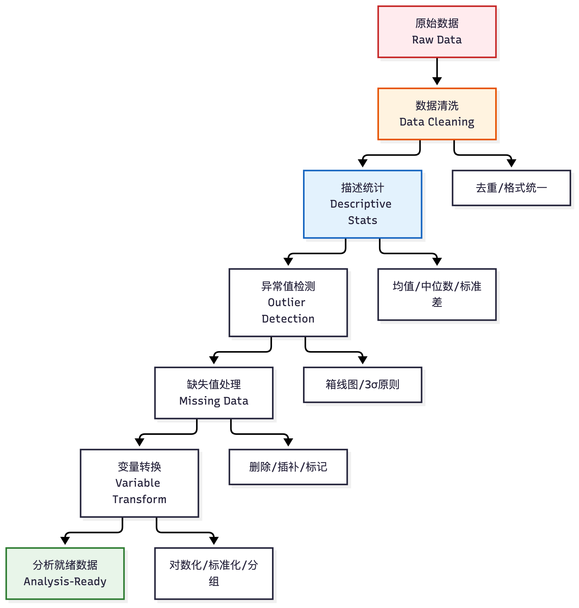
图 8.1 数据体检三步流水线——缺失检查 → 异常值检查 → 缩尾处理,全部动作留痕(S8.1)。
S8.1 留痕要求
上面三步流水线的每一步,都要落到一个可回放的 do 文件里:清理、转换、缩尾各有对应代码,从原始数据一键跑到分析数据。完整的检查点清单与违规示例(含“论文写 N=387、代码跑出 N=392”这类典型对不上)见本章末尾 AI 诚信栏 S8.1,此处不重复列。
§8.3 一元分析
集中趋势
表 8.2 集中趋势。
L4|L4|L4|L4
统计量 & 含义 & 适用场景 & Stata 命令
均值 (Mean) & 所有值的算术平均 & 连续变量、近似正态 & summarize
中位数 (Median) & 排序后中间值 & 偏态分布(如收入) & summarize, detail
众数 (Mode) & 出现频率最高的值 & 分类变量 & tab\
* -- 集中趋势 --
summarize income age df_mean          // 默认输出:N/均值/标准差/最小/最大
summarize income, detail              // 扩展:含中位数/四分位/偏度/峰度
tab gender                            // 分类变量的频数分布(含众数信息)
离散程度
表 8.3 离散程度。
L3|L3|L3
统计量 & 含义 & 特点
极差 (Range) & 最大值 − 最小值 & 对极端值极敏感
标准差 (SD) & 各值偏离均值的平均程度 & 最常用,假设近似正态
方差 (Variance) & SD 的平方 & 回归分析中更常见
四分位距 (IQR) & P75 − P25 & 稳健,不受极端值影响
变异系数 (CV) & SD / Mean & 无量纲,可跨变量比较\
* -- 离散程度 --
summarize income, detail
* 输出中包含:
*   Std. dev.  = 标准差
*   Variance   = 方差
*   Range      = 极差(Max - Min)
*   P25, P50, P75 -> IQR = P75 - P25

* 计算变异系数
quietly summarize income
di "CV = " r(sd)/r(mean)
分布形态
* -- 分布可视化 --

* 直方图
histogram income, frequency normal ///
    title("家庭年收入分布") ///
    xtitle("收入(元)") ytitle("频数") ///
    note("虚线为正态拟合曲线")

* 核密度图(KDE)
kdensity income, title("家庭年收入核密度估计") ///
    xtitle("收入(元)") ytitle("密度")

* 箱线图(识别异常值)
graph box income, title("家庭年收入箱线图") ///
    ytitle("收入(元)") marker(1, size(small))

* Q-Q 正态概率图(目测正态性)
qnorm income, title("收入的正态 Q-Q 图") ///
    xtitle("正态理论分位数") ytitle("样本分位数")

* 偏度与峰度
sktest income                 // Skewness-Kurtosis 联合检验
* H0:服从正态分布;p < 0.05 则拒绝->非正态
swilk income               // Shapiro-Wilk 检验(样本 < 2000 推荐)
* H0:服从正态分布
分类变量的频数分析
* -- 分类变量 --
tab gender                         // 单变量频数
tab gender, nolabel                // 显示数值而非标签
tab income_group                   // 收入分组的频数分布
tab1 gender education income_group // 多个分类变量一次性输出

* 带百分比的频数表
tab income_group, sort             // 按频率排序
综合示例:你的数据“长什么样”
* -- 数据概览(论文 Table 1 的前身)--
* 连续变量
summarize age income df_mean ca_mean, detail

* 分类变量
tab gender
tab education
tab income_group

* 一次性生成描述统计表
tabstat age income df_mean ca_mean, ///
    statistics(n mean sd min p25 p50 p75 max) ///
    columns(statistics) format(%9.2f)
§8.4 双变量分析
相关分析
相关系数衡量两个连续变量之间线性关系的强度和方向:
表 8.4 相关分析。
L2|L2
r 值范围 & 强度判断
* -- Pearson 相关 --
correlate df_mean ca_mean income     // 简单相关
pwcorr df_mean ca_mean income, sig   // 两两相关 + 显著性
pwcorr df_mean ca_mean income, sig star(0.05)  // 标注显著性星号

* 输出解读:
*   r = 0.65, p = 0.000 -> 中等偏强的正相关,在 1% 水平显著
*   注意:相关 ≠ 因果!(第 4 章已强调)

* -- Spearman 秩相关(非正态分布时使用)--
spearman df_mean ca_mean             // 基于排序的相关
* 适用于:有序变量 / 严重偏态 / 有异常值

* -- 相关矩阵热力图 --
* 需要安装:ssc install corrtex
* 或使用 pwcorr 的输出手动制图
交叉表(列联表)
交叉表展示两个分类变量的联合分布:
* -- 基本交叉表 --
tab gender income_group              // 频数
tab gender income_group, row         // 行百分比
tab gender income_group, col         // 列百分比
tab gender income_group, row chi2    // 行百分比 + 卡方检验
tab gender income_group, row chi2 expected  // 含期望频数

* -- 卡方检验解读 --
* H0:两个变量独立(无关联)
* p < 0.05 -> 拒绝 H0 -> 两变量存在显著关联
* 注意:期望频数 < 5 的单元格 > 20% 时,卡方检验不可靠
*       -> 使用 Fisher 精确检验:
tab gender income_group, exact

* -- 多组对比 --
table income_group gender, stat(freq) stat(rowpercent)
组间均值差检验
当你想知道“不同组的连续变量均值是否有显著差异”时:
* -- 两组比较:独立样本 t 检验 --
* 例:男女的数字金融使用是否有显著差异?
ttest df_mean, by(gender)

* 输出解读:
*   看 "diff" 行:均值差 = 男 - 女
*   看 p 值:Pr(|T| > |t|) -> 双尾 p
*   p < 0.05 -> 差异显著
* -- 多组比较:单因素方差分析(ANOVA)--
* 例:不同教育程度的数字金融使用是否有显著差异?
oneway df_mean education_group
* 输出解读:F 统计量与 Pr > F(p < 0.05 则组间差异显著)

* -- 方差不齐时:Welch 校正 --
ttest df_mean, by(gender) welch
* 或:oneway df_mean education_group, welch

* -- 非参数替代(不满足正态假设时)--
* 两组:Mann-Whitney U 检验
ranksum df_mean, by(gender)
* 多组:Kruskal-Wallis 检验
kwallis df_mean, by(education_group)

* -- 效应量 --
* Cohen's d(两组):
* d = (M1 - M2) / Sp,其中 Sp 为合并标准差
* 判断:0.2 = 小效应;0.5 = 中效应;0.8 = 大效应
双变量散点图
* -- 散点图 + 拟合线 --
twoway (scatter df_mean income) ///
       (lfit df_mean income), ///
       title("数字金融使用与收入的关系") ///
       xtitle("家庭年收入(元)") ///
       ytitle("数字金融使用(均值)") ///
       note("实线为 OLS 拟合线")

* 分组散点图
twoway (scatter df_mean income if gender==1, mcolor(blue)) ///
       (scatter df_mean income if gender==2, mcolor(red)) ///
       (lfit df_mean income if gender==1, lcolor(blue)) ///
       (lfit df_mean income if gender==2, lcolor(red)), ///
       legend(label(1 "男") label(2 "女")) ///
       title("数字金融使用与收入(分性别)")
§8.5 描述表三线表输出
什么是三线表?
三线表 = 顶线 + 栏目线 + 底线,无竖线。这是国际学术期刊的通行格式:
----------------------------------------------
变量          观测值   均值    标准差   最小值   最大值
----------------------------------------------
年龄          387     42.35    12.18    18      78
家庭年收入    385     56,230   32,450   3,000   280,000
数字金融使用  387      3.42     0.89     1.00    5.00
信贷可得性    380      3.18     0.95     1.00    5.00
----------------------------------------------
注:数据来源于作者调查。收入单位为元/年。
----------------------------------------------
方法一:esttab(推荐,适合复杂表格)
* -- 安装(首次使用)--
* ssc install estout

* -- 生成描述统计表 --
* 步骤 1:用 postfile 手动构建
capture postclose desc_tab
tempname desc_tab
postfile `desc_tab' str20 varname n mean sd min max using "desc_tab.dta", replace
* 步骤 2:逐个变量计算并写入
foreach v of varlist age income df_mean ca_mean {
    quietly summarize `v', detail
    post `desc_tab' ("`v'") (r(N)) (r(mean)) (r(sd)) (r(min)) (r(max))
}
postclose `desc_tab'

* 步骤 3:读回并输出为 LaTeX 表格
use "desc_tab.dta", clear
listtab latex, style(booktabs) ///
    head("\toprule" "变量 & N & 均值 & 标准差 & 最小值 & 最大值 \\ \midrule") ///
    foot("\hline") ///
    begin("") end(" \\\\") delimiter(" & ")
* 注意:listtab 需要 ssc install listtab
方法二:tabstat + putexcel(简单直接)
* -- 方法二:tabstat 输出到 Excel --
* 步骤 1:生成描述统计
tabstat age income df_mean ca_mean, ///
    statistics(n mean sd min max) ///
    columns(statistics) format(%9.2f) ///
    save
* save 选项将结果存入 r(StatMat) 矩阵

* 步骤 2:导出到 Excel
matrix stats = r(StatMat)'
putexcel set "table1_descriptive.xlsx", replace
putexcel A1 = "变量" B1 = "观测值" C1 = "均值" D1 = "标准差" E1 = "最小值" F1 = "最大值"
putexcel A2 = matrix(stats)
putexcel close
方法三:putdocx(直接生成 Word 文档)
* -- 方法三:putdocx 生成三线表 --
capture putdocx clear
putdocx begin

* 标题
putdocx paragraph, style(Heading2)
putdocx text("表 1  主要变量描述性统计")

* 创建表格(5 变量 × 6 列 = 变量名 + 5 个统计量)
putdocx paragraph
putdocx table tbl1 = (6, 6), border(bottom, none) border(top, none)

* 表头
putdocx table tbl1(1,1) = ("变量"), bold
putdocx table tbl1(1,2) = ("N"), bold
putdocx table tbl1(1,3) = ("均值"), bold
putdocx table tbl1(1,4) = ("标准差"), bold
putdocx table tbl1(1,5) = ("最小值"), bold
putdocx table tbl1(1,6) = ("最大值"), bold

* 填充数据(循环写入)
local row = 2
foreach v of varlist age income df_mean ca_mean {
    quietly summarize `v', detail
    putdocx table tbl1(`row',1) = ("`v'")
    putdocx table tbl1(`row',2) = (r(N)), fmt("0")
    putdocx table tbl1(`row',3) = (r(mean)), fmt("%9.2f")
    putdocx table tbl1(`row',4) = (r(sd)), fmt("%9.2f")
    putdocx table tbl1(`row',5) = (r(min)), fmt("%9.2f")
    putdocx table tbl1(`row',6) = (r(max)), fmt("%9.2f")
    local ++row
}

* 添加三线表样式(顶线、表头底线、底线)
putdocx table tbl1, border(top, single, black, 1.5pt)
putdocx table tbl1(1,.), border(bottom, single, black, 0.75pt)
putdocx table tbl1(6,.), border(bottom, single, black, 1.5pt)
putdocx save "table1_descriptive.docx", replace
putdocx close
di "描述统计表已导出至 table1_descriptive.docx"
方法四:esttab 一键输出(最简方案)
* -- 最简方案:esttab 描述统计 --
* 需要:ssc install estout

* 先用 estpost 存储描述统计
estpost summarize age income df_mean ca_mean, detail
* 或:
estpost tabstat age income df_mean ca_mean, ///
    statistics(count mean sd min max) columns(statistics)

* 导出三线表
esttab using "table1.rtf", replace ///
    cells("count(fmt(0) label(观测值)) mean(fmt(2) label(均值)) sd(fmt(2) label(标准差)) min(fmt(2) label(最小值)) max(fmt(2) label(最大值))") ///
    noobs nomtitle nonumber ///
    title("表 1  主要变量描述性统计") ///
    addnotes("注:数据来源于作者调查。") ///
    label booktabs
* booktabs 选项 -> 三线表格式
分组描述表(论文常见 Table 1 变体)
* -- 按组报告描述统计 + 均值差检验 --
* 例:按性别分组
estpost ttest age income df_mean ca_mean, by(gender)

esttab using "table1_by_gender.rtf", replace ///
    cells("mu_1(fmt(2) label(男性均值)) mu_2(fmt(2) label(女性均值)) b(fmt(2) label(差异)) p(fmt(3) label(p值))") ///
    noobs nomtitle nonumber ///
    title("表 1  描述性统计(按性别分组)") ///
    addnotes("注:*** p<0.01, ** p<0.05, * p<0.1") ///
    label booktabs
AI 辅助研究栏 · 第 8 章
AI 在描述统计中的合法应用
表 8.5 AI 在描述统计中的合法应用。
L3|L3|L3
应用场景 & 具体做法 & 注意事项
代码生成 & 告诉 AI 你的变量名和需求,让它生成 Stata 代码 & 运行前检查语法和逻辑
输出解读 & 将 summarize, detail 输出贴给 AI,让它帮你判断分布特征 & 理解比背诵重要
异常值诊断 & 贴入极端值让 AI 分析可能原因 & 不能因为“不合理”就删除——需有依据
表格美化 & 让 AI 帮你把 esttab 输出调整为期刊要求的格式 & 格式可以 AI 辅助,数据不能 AI 编造
缺失值策略选择 & 描述你的数据缺失情况,让 AI 推荐策略 & 最终决策需结合理论和文献\
AI 不能做的事
❌ 替你编造描述统计数据(论文中的每一个数字都必须来自真实运行结果)
❌ 帮你“美化”异常值使其“看起来合理”
❌ 替代你对数据质量的判断——AI 没有看过你的原始问卷
AI 诚信栏 · 第 8 章
S8.1 数据处理全留痕可复现
+-----------------------------------------------------+
|  * 诚信检查点 S8.1                                    |
|                                                       |
|  核心原则:                                            |
|  从原始数据到论文中任何一张表格,中间的每一步操作        |
|  都必须有代码记录,且他人可按你的代码完整复现。          |
|                                                       |
|  具体要求:                                            |
|  1. 每步操作(清洗、变量生成、合并)都写在 do 文件中    |
|  2. 不使用 clear 后手动输入数据的方式                   |
|  3. 所有随机种子用 set seed 固定(如 set seed 20260601)|
|  4. 运行 log 文件保存完整输出(log using ...)          |
|  5. 论文中的样本量、均值等必须与 log 可交叉验证        |
|                                                       |
|  常见"翻车"场景:                                      |
|  · 论文报告 N=387,但 do 文件跑出来是 N=392           |
|  · 表格中的数字与 log 文件不一致                       |
+-----------------------------------------------------+
本章产出物
表 8.6 本章产出物。
L4|L4|L4|L4
序号 & 产出物 & 文件名建议 & 说明
1 & 数据准备脚本 & 02_clean.do & 从原始到分析数据的全过程
2 & 数据体检报告 & & 缺失/异常值/缩尾记录
3 & 描述统计表 & & 三线表格式
4 & 分析数据集 & analysis_data.dta & 清洗完毕、可直接跑回归\
下一章预告:第 9 章进入实证分析的核心——回归模型的设定、估计与诊断。你的描述统计做扎实了,回归才能跑得放心。
English Edition
Chapter 8 · Descriptive Statistics and the Data Health Check
Chapter Overview
Learning Objectives
After completing this chapter, you will be able to:
The four steps of data preparation—cleaning, missing-value handling, variable transformation, weighting
The three steps of the data health check—missing check, outlier check, winsorization (all logged and reproducible)
Univariate analysis—central tendency (mean/median/mode), dispersion (SD/range/IQR), distribution shape
Bivariate analysis—correlation, cross-tabs, tests of between-group mean differences
Descriptive tables in three-line style—the Stata implementation of the academic standard
Chapter Roadmap
Data enters the warehouse (Ch. 7)
      v
8.1 Data preparation, four steps
      v
8.2 Data health check, three steps (logged per S8.1)
      v
8.3 Univariate -> 8.4 Bivariate analysis
      v
8.5 Descriptive tables in three-line style
      v
Ready for Ch. 9's regression work
8.1 Data Preparation in Four Steps
Step 1: Data Cleaning
* -- Data cleaning --
clear all
set more off
use "survey_clean.dta", clear

* Check duplicate observations
duplicates report
duplicates drop id, force   // deduplicate by ID

* Check that variable types are correct
describe
* Common problem: numbers read as strings (spaces or special
* characters in the Excel source)
destring age income, replace force  // force conversion

* Eye-scan the first 20 rows
list id gender age income in 1/20
Step 2: Handling Missing Values
Three strategies were introduced earlier; here is the Stata implementation:
Table 8.1 Step 2: handling missing values.
L4|L4|L4|L4
Strategy & When to use & Advantage & Drawback
Listwise deletion & Little missingness (
Mean/median imputation & Little missingness, near-normal & Preserves sample size & Understates variance
Multiple imputation (MI) & Much missingness (
* -- Missing-value diagnostics --
* Missingness per variable
misstable summarize

* Missingness patterns
misstable patterns

* -- Strategy 1: listwise deletion (Stata's default) --
* Nothing extra needed; regress and friends use listwise
* deletion automatically
* Verify: observations used are in e(sample)
regress y x1 x2 x3
di "Regression sample size: " e(N)

* -- Strategy 2: mean/median imputation --
* Mean imputation (near-normal variables)
summarize income
replace income = r(mean) if missing(income)

* Median imputation (skewed variables such as income)
summarize income, detail
replace income = r(p50) if missing(income)

* -- Strategy 3: multiple imputation (recommended if > 5%) --
mi register imputed income age
mi impute chained (regress) income age = gender education df1-df5, add(5)
mi estimate: regress y x1 x2 x3
Step 3: Variable Transformation
* -- Reverse-scored items --
* Reverse a Likert 1-5 item: new = 6 - old
gen df2_r = 6 - df2
label var df2_r "Digital finance use 2 (reversed)"

* -- Construct scores: sum or mean --
* Option A: mean (recommended; unaffected by item count)
egen df_mean = rowmean(df1 df2_r df3 df4 df5)
label var df_mean "Digital finance use (mean)"

* Option B: sum
egen df_sum = rowtotal(df1 df2_r df3 df4 df5)
label var df_sum "Digital finance use (sum)"

* Check the correlation of the two (usually > 0.95)
correlate df_mean df_sum

* -- Standardized variables (optional; comparable betas) --
foreach var of varlist income df_mean ca_mean {
    quietly summarize `var'
    gen `var'_z = (`var' - r(mean)) / r(sd)
    label var `var'_z "`var' (standardized)"
}

* -- Log transformation (common for skewed variables) --
gen ln_income = ln(income)
label var ln_income "Household annual income (log)"

* -- Dummy variables --
tab gender, gen(gender_d)
* gender_d1 = male, gender_d2 = female -> use gender_d1 in
* regressions
Step 4: Weighting
* -- Survey weights (complex sampling designs) --
* If you used stratified sampling, tell Stata the weights
svyset psu [pweight = weight], strata(strata)

* Prefix later analyses with svy:
svy: mean income
svy: regress y x1 x2

* Without a complex design (simple random or convenience
* sampling), usually no weighting
8.2 The Data Health Check in Three Steps
Core idea: before running any regression, give the data a full physical examination—finding problems beats pretending there are none.
Step 1: Missing Check
* -- Full missingness diagnosis --
* Method 1: proportion missing per variable
foreach var of varlist _all {
    quietly count if missing(`var')
    if r(N) > 0 {
        di "`var'" _col(30) "missing " r(N) " (" %5.2f r(N)/_N*100 "%)"
    }
}

* Method 2: the misstable family
misstable summarize          // summary table
misstable summarize, by(gender)  // is missingness systematic?
misstable patterns           // which variables go missing together
misstable tree               // missingness decision tree
Decision standards:
Per-variable missingness
5%: usually delete or mean-impute Per-variable missingness 5–20%: prefer multiple imputation
Per-variable missingness
20%: question whether the variable is usable Systematic missingness (e.g., high earners less likely to report income): must be discussed in the paper
Step 2: Outlier Check
* -- Outlier diagnostics --

* Method 1: scan basic statistics
summarize income age df_mean, detail
* Watch: are max/min plausible? Is the mean dragged by
* extremes?

* Method 2: box plot (visualization)
graph box income, over(gender) title("Income by gender")
* Method 3: the IQR rule flags outliers automatically
quietly summarize income, detail
local p25 = r(p25)
local p75 = r(p75)
local iqr = `p75' - `p25'
local lower = `p25' - 1.5 * `iqr'
local upper = `p75' + 1.5 * `iqr'
gen outlier_income = (income < `lower' | income > `upper')
tab outlier_income

* Flag outliers for many variables (foreach loop)
foreach var of varlist income age df_mean {
    quietly summarize `var', detail
    local p1 = r(p1)
    local p99 = r(p99)
    count if `var' < `p1' | `var' > `p99'
    di "  Obs beyond 1%-99%: " r(N)
}
Step 3: Winsorization
* -- Winsorization --
* Install the community command (first use)
* ssc install winsor2

* Winsorize all continuous variables at 1%/99%
winsor2 income age df_mean ca_mean, replace cuts(1 99)

* Before/after comparison
* Save pre-winsor statistics first
summarize income, detail
local pre_mean = r(mean)
local pre_sd   = r(sd)
local pre_min  = r(min)
local pre_max  = r(max)

* Winsorize
winsor2 income, replace cuts(1 99)

* Compare
summarize income, detail
di "=== Income, before vs. after winsorizing ==="
di "  Before: mean=" `pre_mean' " sd=" `pre_sd' " min=" `pre_min' " max=" `pre_max'
di "  After:  mean=" r(mean)    " sd=" r(sd)    " min=" r(min)    " max=" r(max)
di "Method: winsor2, 1% two-tailed"
di "Reason: extreme values threatened regression robustness"
log close
Figure 8.1 The three-step health-check pipeline—missing check → outlier check → winsorization, every action logged (S8.1).
The S8.1 Logging Requirement
Every step of the three-step pipeline above must land in a replayable do file: cleaning, transformation, and winsorization each have their code, and the raw data runs to the analysis data in one click. The full checkpoint list and violation examples (including the classic “paper says N=387 but the code yields N=392” mismatch) appear in the AI Integrity Corner S8.1 at the end of this chapter and are not repeated here.
8.3 Univariate Analysis
Central Tendency
Table 8.2 Central tendency.
L4|L4|L4|L4
Statistic & Meaning & When to use & Stata command
Mean & Arithmetic average of all values & Continuous, near-normal & summarize
Median & Middle value after sorting & Skewed distributions (e.g., income) & summarize, detail
Mode & Most frequent value & Categorical variables & tab\
* -- Central tendency --
summarize income age df_mean          // N, mean, SD, min, max
summarize income, detail              // adds median/quartiles/skew/kurtosis
tab gender                            // frequency distribution (mode info)
Dispersion
Table 8.3 Dispersion.
L3|L3|L3
Statistic & Meaning & Features
Range & Max
Standard deviation (SD) & Average deviation from the mean & Most common; assumes near-normality
Variance & SD squared & More common in regression work
Interquartile range (IQR) & P75
Coefficient of variation (CV) & SD / Mean & Unit-free; comparable across variables\
* -- Dispersion --
summarize income, detail
* The output includes:
*   Std. dev.
*   Variance
*   Range (Max - Min)
*   P25, P50, P75 -> IQR = P75 - P25

* Coefficient of variation
quietly summarize income
di "CV = " r(sd)/r(mean)
Distribution Shape
* -- Distribution visualization --

* Histogram
histogram income, frequency normal ///
    title("Household annual income") ///
    xtitle("Income (CNY)") ytitle("Frequency") ///
    note("Dashed line: normal fit")

* Kernel density (KDE)
kdensity income, title("Kernel density of income") ///
    xtitle("Income (CNY)") ytitle("Density")

* Box plot (outlier detection)
graph box income, title("Box plot of income") ///
    ytitle("Income (CNY)") marker(1, size(small))

* Q-Q normal plot (eyeball normality)
qnorm income, title("Normal Q-Q plot of income") ///
    xtitle("Normal theoretical quantiles") ytitle("Sample quantiles")

* Skewness and kurtosis
sktest income                 // joint Skewness-Kurtosis test
* H0: normal; p < 0.05 rejects -> non-normal
swilk income               // Shapiro-Wilk (recommended if n < 2000)
* H0: normal
Frequency Analysis of Categorical Variables
* -- Categorical variables --
tab gender                         // univariate frequencies
tab gender, nolabel                // show values, not labels
tab income_group                   // frequencies of income groups
tab1 gender education income_group // several at once

* Frequency table with percentages
tab income_group, sort             // sorted by frequency
Worked Overview: What Your Data “Looks Like”
* -- Data overview (precursor of the paper's Table 1) --
* Continuous variables
summarize age income df_mean ca_mean, detail

* Categorical variables
tab gender
tab education
tab income_group

* One-shot descriptive table
tabstat age income df_mean ca_mean, ///
    statistics(n mean sd min p25 p50 p75 max) ///
    columns(statistics) format(%9.2f)
8.4 Bivariate Analysis
Correlation Analysis
The correlation coefficient measures the strength and direction of the linear relationship between two continuous variables:
Table 8.4 Correlation analysis.
L2|L2
Range of
* -- Pearson correlation --
correlate df_mean ca_mean income     // simple correlation
pwcorr df_mean ca_mean income, sig   // pairwise + significance
pwcorr df_mean ca_mean income, sig star(0.05)  // with stars

* Reading the output:
*   r = 0.65, p = 0.000 -> moderately strong positive,
*   significant at 1%
*   Caution: correlation is NOT causation! (Ch. 4)

* -- Spearman rank correlation (non-normal data) --
spearman df_mean ca_mean             // rank-based correlation
* For: ordinal variables / heavy skew / outliers

* -- Correlation heatmap --
* Install: ssc install corrtex
* or plot manually from pwcorr output
Cross-Tabs (Contingency Tables)
Cross-tabs show the joint distribution of two categorical variables:
* -- Basic cross-tabs --
tab gender income_group              // counts
tab gender income_group, row         // row percentages
tab gender income_group, col         // column percentages
tab gender income_group, row chi2    // row % + chi-squared
tab gender income_group, row chi2 expected  // with expected counts

* -- Reading the chi-squared test --
* H0: the two variables are independent (no association)
* p < 0.05 -> reject H0 -> significant association
* Caution: if cells with expected count < 5 exceed 20%,
* the chi-squared test is unreliable
*       -> use Fisher's exact test:
tab gender income_group, exact

* -- Multi-group comparison --
table income_group gender, stat(freq) stat(rowpercent)
Tests of Between-Group Mean Differences
When you want to know whether group means of a continuous variable differ significantly:
* -- Two groups: independent-samples t test --
* Example: do men and women differ in digital finance use?
ttest df_mean, by(gender)

* Reading the output:
*   The "diff" row: mean difference = male - female
*   The p value: Pr(|T| > |t|) -> two-tailed p
*   p < 0.05 -> significant difference
* -- Many groups: one-way ANOVA --
* Example: does use differ across education levels?
oneway df_mean education_group
* Reading: F statistic and Pr > F (p < 0.05 -> differences)

* -- Unequal variances: Welch correction --
ttest df_mean, by(gender) welch
* or: oneway df_mean education_group, welch

* -- Non-parametric alternatives (normality violated) --
* Two groups: Mann-Whitney U
ranksum df_mean, by(gender)
* Many groups: Kruskal-Wallis
kwallis df_mean, by(education_group)

* -- Effect size --
* Cohen's d (two groups):
* d = (M1 - M2) / Sp, Sp = pooled SD
* Benchmarks: 0.2 small; 0.5 medium; 0.8 large
Bivariate Scatter Plots
* -- Scatter + fitted line --
twoway (scatter df_mean income) ///
       (lfit df_mean income), ///
       title("Digital finance use and income") ///
       xtitle("Household annual income (CNY)") ///
       ytitle("Digital finance use (mean)") ///
       note("Solid line: OLS fit")

* Grouped scatter
twoway (scatter df_mean income if gender==1, mcolor(blue)) ///
       (scatter df_mean income if gender==2, mcolor(red)) ///
       (lfit df_mean income if gender==1, lcolor(blue)) ///
       (lfit df_mean income if gender==2, lcolor(red)), ///
       legend(label(1 "Male") label(2 "Female")) ///
       title("Digital finance use and income, by gender")
8.5 Descriptive Tables in Three-Line Style
What Is a Three-Line Table?
Three lines = top rule + header rule + bottom rule, no vertical rules—the standard format of international journals:
----------------------------------------------
Variable        Obs     Mean      SD      Min       Max
----------------------------------------------
Age             387    42.35    12.18      18        78
Hh income/yr    385  56,230   32,450   3,000   280,000
Dig. finance    387     3.42     0.89    1.00     5.00
Credit access   380     3.18     0.95    1.00     5.00
----------------------------------------------
Note: authors' survey. Income in CNY/year.
----------------------------------------------
Method 1: esttab (Recommended for Complex Tables)
* -- Install (first use) --
* ssc install estout

* -- Build the descriptive table --
* Step 1: construct manually with postfile
capture postclose desc_tab
tempname desc_tab
postfile `desc_tab' str20 varname n mean sd min max using "desc_tab.dta", replace
* Step 2: compute and write variable by variable
foreach v of varlist age income df_mean ca_mean {
    quietly summarize `v', detail
    post `desc_tab' ("`v'") (r(N)) (r(mean)) (r(sd)) (r(min)) (r(max))
}
postclose `desc_tab'

* Step 3: read back and emit a LaTeX table
use "desc_tab.dta", clear
listtab latex, style(booktabs) ///
    head("\toprule" "Variable & N & Mean & SD & Min & Max \\ \midrule") ///
    foot("\hline") ///
    begin("") end(" \\\\") delimiter(" & ")
* Note: listtab requires ssc install listtab
Method 2: tabstat + putexcel (Simple and Direct)
* -- Method 2: tabstat to Excel --
* Step 1: compute the statistics
tabstat age income df_mean ca_mean, ///
    statistics(n mean sd min max) ///
    columns(statistics) format(%9.2f) ///
    save
* save stores the results in the r(StatMat) matrix

* Step 2: export to Excel
matrix stats = r(StatMat)'
putexcel set "table1_descriptive.xlsx", replace
putexcel A1 = "Variable" B1 = "Obs" C1 = "Mean" D1 = "SD" E1 = "Min" F1 = "Max"
putexcel A2 = matrix(stats)
putexcel close
Method 3: putdocx (Word Document Directly)
* -- Method 3: putdocx three-line table --
capture putdocx clear
putdocx begin

* Title
putdocx paragraph, style(Heading2)
putdocx text("Table 1  Descriptive statistics of key variables")

* Create the table (6 rows x 6 cols)
putdocx paragraph
putdocx table tbl1 = (6, 6), border(bottom, none) border(top, none)

* Header
putdocx table tbl1(1,1) = ("Variable"), bold
putdocx table tbl1(1,2) = ("N"), bold
putdocx table tbl1(1,3) = ("Mean"), bold
putdocx table tbl1(1,4) = ("SD"), bold
putdocx table tbl1(1,5) = ("Min"), bold
putdocx table tbl1(1,6) = ("Max"), bold

* Fill the data (loop)
local row = 2
foreach v of varlist age income df_mean ca_mean {
    quietly summarize `v', detail
    putdocx table tbl1(`row',1) = ("`v'")
    putdocx table tbl1(`row',2) = (r(N)), fmt("0")
    putdocx table tbl1(`row',3) = (r(mean)), fmt("%9.2f")
    putdocx table tbl1(`row',4) = (r(sd)), fmt("%9.2f")
    putdocx table tbl1(`row',5) = (r(min)), fmt("%9.2f")
    putdocx table tbl1(`row',6) = (r(max)), fmt("%9.2f")
    local ++row
}

* Three-line styling (top, header, bottom rules)
putdocx table tbl1, border(top, single, black, 1.5pt)
putdocx table tbl1(1,.), border(bottom, single, black, 0.75pt)
putdocx table tbl1(6,.), border(bottom, single, black, 1.5pt)
putdocx save "table1_descriptive.docx", replace
putdocx close
di "Descriptive table exported to table1_descriptive.docx"
Method 4: esttab One-Shot Export (Simplest)
* -- Simplest: esttab for descriptive statistics --
* Requires: ssc install estout

* Store the statistics with estpost first
estpost summarize age income df_mean ca_mean, detail
* or:
estpost tabstat age income df_mean ca_mean, ///
    statistics(count mean sd min max) columns(statistics)

* Export the three-line table
esttab using "table1.rtf", replace ///
    cells("count(fmt(0) label(Obs)) mean(fmt(2) label(Mean)) sd(fmt(2) label(SD)) min(fmt(2) label(Min)) max(fmt(2) label(Max))") ///
    noobs nomtitle nonumber ///
    title("Table 1  Descriptive statistics of key variables") ///
    addnotes("Note: authors' survey.") ///
    label booktabs
* the booktabs option -> three-line style
Grouped Descriptive Tables (The Common Table 1 Variant)
* -- Grouped statistics + mean-difference test --
* Example: grouped by gender
estpost ttest age income df_mean ca_mean, by(gender)

esttab using "table1_by_gender.rtf", replace ///
    cells("mu_1(fmt(2) label(Male mean)) mu_2(fmt(2) label(Female mean)) b(fmt(2) label(Difference)) p(fmt(3) label(p-value))") ///
    noobs nomtitle nonumber ///
    title("Table 1  Descriptive statistics by gender") ///
    addnotes("Note: *** p<0.01, ** p<0.05, * p<0.1") ///
    label booktabs
AI-Assisted Research Corner · Chapter 8
Legitimate AI Uses in Descriptive Statistics
Table 8.5 Legitimate AI uses in descriptive statistics.
L3|L3|L3
Use case & How & Caveat
Code generation & Tell AI your variable names and needs; it drafts Stata code & Check syntax and logic before running
Output interpretation & Paste summarize, detail output; AI helps characterize the distribution & Understanding beats memorization
Outlier diagnosis & Paste extreme values; AI suggests possible causes & Never delete just because “it looks wrong”—you need grounds
Table formatting & AI adjusts esttab output to journal format & AI may help format; it must never fabricate data
Missing-value strategy & Describe your missingness; AI recommends a strategy & The final decision needs theory and literature\
What AI Must Not Do
❌ Fabricate descriptive statistics for you (every number in the paper must come from a real run)
❌ “Beautify” outliers until they “look plausible”
❌ Replace your judgment of data quality—AI has never seen your raw questionnaires
AI Integrity Corner · Chapter 8
S8.1 Full Logging and Reproducibility of Data Processing
+-----------------------------------------------------+
|  * Integrity checkpoint S8.1                        |
|                                                     |
|  Core principle:                                    |
|  Every operation between the raw data and any table |
|  in the paper must be recorded in code, and others  |
|  must be able to reproduce it fully from your code. |
|                                                     |
|  Requirements:                                      |
|  1. Every step (cleaning, variables, merges) lives  |
|     in a do-file                                    |
|  2. No manual data entry after clear                |
|  3. All random seeds fixed with set seed            |
|     (e.g., set seed 20260601)                       |
|  4. A log file captures the full output             |
|     (log using ...)                                 |
|  5. Sample sizes, means, etc. in the paper must     |
|     cross-check against the log                     |
|                                                     |
|  Classic failures:                                  |
|  - Paper reports N=387; the do-file yields N=392    |
|  - Table numbers disagree with the log file         |
+-----------------------------------------------------+
Chapter Deliverables
Table 8.6 Chapter deliverables.
L4|L4|L4|L4
# & Deliverable & Suggested filename & Description
1 & Data preparation script & 02_clean.do & Raw to analysis data, the whole path
2 & Data health report & & Missing / outliers / winsorization record
3 & Descriptive table & & Three-line style
4 & Analysis dataset & analysis_data.dta & Cleaned, ready for regressions\
Next chapter preview: Chapter 9 enters the core of empirical analysis—specification, estimation, and diagnostics of regression models. Only on solid descriptive work can regressions run with confidence.