📖 《把 AI 当助手——经济实证研究的诚信、方法与工具》双语网页版:每章中文部在前,English Edition 在后,内容与最新合订 PDF 一致。
第4章 · 研究设计
学习目标
完成本章后,你应当能够:
说出内部效度七大威胁(历史 / 成熟 / 测验效应 / 仪器变化 / 统计回归 / 选择偏差 / 样本流失),并各配 1 个金融版例子
区分三大设计类型(真实验 / 准实验 / 非实验—事后追溯),并判断自己的研究属于哪一类
用“相关≠因果”三个金融故事,解释遗漏变量、反向因果与选择偏差
写出
research_design.md五栏方案(问题 / 理论 / 假说 / 数据 / 方法)
[提示] 本章篇幅不长,但它是全手册的“承重墙”。第 9 章所有识别策略(IV / DID / PSM / RDD / FE),本质上都在回答本章提出的那个问题:你凭什么说 X 导致了 Y?
§4.1 研究问题三类型
📐 结构图示(书版示意图的文字要点)
- tikzpicture
- ->,very thick,NavyBlue
- 探索型
- What is going on?
- 例:
- 方法:
- 样本:
- 产出:
图 4.1 研究问题三类型——并列不是选项,而是递进的三层:先把现象摸清,再量化测度,最后识别因果。
三类型是递进的三层,不是并列的三个选项
描述型   ->   相关型   ->   因果型
(知道有什么)(知道有关联)(知道谁导致谁)

   证据强度 ^     方法难度 ^     数据要求 ^     工作量 ^
没有描述就直接谈因果,读者不知道你的样本长什么样
没有相关就直接谈因果,你连“值不值得深挖”都不知道
但只停在描述和相关,好期刊发不了——审稿人会问一句“So what?”
类型决定方法
表 4.1 类型决定方法。
L3|L3|L3
你的问题类型 & 最低方法要求 & 落到手册哪一章
描述型 & 代表性样本 + 规范统计报告 + 合理的指标体系 & 第 5 章(抽样)+ 第 8 章(描述统计)
相关型 & 回归 + 控制变量 + 显著性检验 & 第 9 章 §9.1(OLS)
因果型 & 识别策略 + 内生性讨论 + 稳健性检验 + 机制检验 & 第 9 章 §9.2—9.7 全套\
△ 最常见的致命错误:问题写成因果型(“数字金融对农户收入的影响”),方法却用相关型(跑一个 OLS 就完事)。这在开题时会被导师打回,在投稿时会被直接拒稿。
两条出路,选一条:
降级问题:把“影响”改成“相关性”——诚实、省力,但贡献也变小
升级方法:找到识别策略(政策冲击 → DID;外生工具 → IV;参与门槛 → RDD)——费力,但这是能发表的路
[提示] 内部效度就是因果关系,它需要三个条件——① 原因和结果相互关联;② 时间优先(原因先于结果发生);③ 没有其他看似合理的解释(无伪相关)。第 9 章的所有方法,都在努力满足 ② 和 ③。
三方向练习
把你第 3 章 one_page_proposal.md 里的研究问题,按三类型各写一遍:
表 4.2 三方向练习。
L4|L4|L4|L4
方向 & 描述型版本 & 相关型版本 & 因果型版本
【农】农村金融 & 四川省农户数字金融使用的现状与分布特征 & 数字金融使用与农户收入是否相关 & 数字金融使用是否提高了农户收入(识别策略:___)
【险】风险管理/保险 & 三大粮食作物完全成本保险试点的覆盖率与赔付情况 & 农业保险参与和农户生产投资是否相关 & 完全成本保险试点是否提高了农户粮食产量(识别策略:DID)
【金】金融理论与政策 & LPR 改革后贷款利率的分布变化 & LPR 变动与企业投资是否相关 & LPR 下调是否通过信贷渠道刺激了企业投资(识别策略:___)\
然后问自己两个问题:我打算做哪一层?我有没有能力做到那一层?
§4.2 内部效度与外部效度:七大威胁
先分清两种效度
表 4.3 先分清两种效度。
L4|L4|L4|L4
效度 & 问的是 & 通俗说法 & 标准定义
内部效度 & X 真的导致了 Y 吗? & “是不是它干的” & 因变量的变化是否确实由假定的自变量造成,而非外生变量引起
外部效度 & 这个结论能推广吗? & “换个人换个地方还成立吗” & 观察到的相关性能否从样本推广到总体(总体效度),或适用于其他人 / 组织 / 情境 / 时间(生态效度)\
[重点] 另外两种效度:构念效度(你的量表真的测到了那个构念吗)和统计结论效度(统计方法用对了吗、前提假设满足吗)。这两种分别在第 5 章和第 9 章详讲。
权衡关系:内部效度与外部效度常存在权衡——实验室实验内部效度高但外部效度低(人为环境不代表真实世界);现场调查外部效度高但内部效度低(无法操控自变量)。经济研究的绝大多数选题,都站在这个权衡的“外部效度较高、内部效度较低”一侧——这正是为什么需要识别策略。
李宝良、郭其友[78]在述评 2021 年诺贝尔经济学奖(Angrist、Imbens、Card)时指出,实证经济学“可信性革命”的核心要义是:因果评估的可信性不依赖数据与计量方法本身,而依赖对自然实验背后制度运作过程的深刻理解。换言之,好的识别策略源于制度知识,而非技术工具——你只有深入理解农业保险的试点遴选机制,才能找到有效的 DID 断点;你只有理解数字金融平台的准入门槛,才能找到自然断点做 RDD。这与 §3.7 选题三问中“能力圈”一问形成呼应:能力圈不只是“我会不会跑 DID/Stata”,更是“我理不理解这个政策/制度的运作逻辑”。初学者常犯的错误是先学了 IV/DID 再找题目——正确顺序恰好相反:先有对制度的深度理解,识别策略才水到渠成。
七大内部效度威胁
表 4.4 七大内部效度威胁。
L4|L4|L4|L4
# & 威胁 & 含义 & 例子
1 & 历史(History) & 观测到的结果由研究期间发生的外部事件而非处理引起 & “你的研究期恰好赶上 LPR 下调 / 疫情 / 房地产调控”——结果变了,但不是你研究的那个 X 干的
2 & 成熟(Maturation) & 结果由被试自身的自然成熟而非处理引起 & “三年面板里农户自己学习、经验积累,金融素养自然提高了”——不是培训的功劳
3 & 测验效应(Testing) & 前测影响后测(被试记住答案或学会应付) & “第一次被问收入后,农户学会了少报(或记住了问卷答案)”——第二轮数据“变好看”了
4 & 仪器变化(Instrumentation) & 前后测量工具或标准发生变化 & “统计口径 2020 年改了”“数字普惠金融指数的编制方法 2021 年调整了”——数据跳变不是现实跳变
5 & 统计回归(Regression to the mean) & 极端值在第二次测量时向均值回归 & “你专挑最穷的村做试点,次年它们自然好转”——不是政策有效,是均值回归
6 & 选择偏差(Selection) & 实验组与对照组先天不等价 & “参加农业保险的都是风险厌恶型农户”“试点县本来就是省里挑的先进县”
7 & 样本流失(Attrition) & 被试系统性退出,且两组流失率不同 & “三年面板中 20% 农户失联,且失联的多数是外出务工、收入变化最大的那批”\
经济研究里最常踩的三个
① 选择偏差——经济研究的头号杀手
任何“自愿参与”的项目都有这个问题:保险、贷款、培训、合作社、数字钱包。愿意参加的人和不愿参加的人从一开始就不一样(风险偏好、能力、财富、社会关系)。
观察:投保农户的平均产量 > 未投保农户
错误推断:农业保险提高了产量
真相可能:产量高、收入稳的农户更有钱也更有动机投保
(即“产量 -> 投保”,而不是“投保 -> 产量”)怎么防:随机分组(RCT,最干净)/ 倾向得分匹配 PSM(匹配可观测特征)/ 工具变量 IV(找外生变化)/ 断点回归 RDD(利用参与门槛)。→ 第 9 章 §9.3、§9.5
② 历史威胁——政策评估的常见陷阱
观察:2020 年数字金融试点县的农民收入增速高于非试点县
错误推断:数字金融试点有效
真相可能:2020 年恰逢脱贫攻坚收官,试点县同时获得了大量其他转移支付怎么防:DID(用对照组吸收共同的时间冲击)+ 平行趋势检验;控制同期其他政策变量;安慰剂检验(把政策时点人为提前,看“效果”是否消失)。→ 第 9 章 §9.4
③ 统计回归——“专挑最差的样本”的必然代价
扶贫、普惠金融项目天然倾向于选“最困难的样本”。而这些极端样本下一期大概率会自然好转——这不是政策效果,是统计规律。
观察:最贫困的 100 户获得小额信贷后,次年收入平均上升 18%
错误推断:小额信贷使收入提高 18%
真相可能:即使不给贷款,这 100 户中很多也会自然回升(均值回归)怎么防:设一个按同样规则筛选的对照组(关键是筛选规则一致);用 DID 而不是简单的前后对比。
外部效度:你的结论能推广多远
内部效度解决了“是不是它干的”,外部效度问“在别的地方也是它干的吗”。三个常见推广障碍:
表 4.5 外部效度:你的结论能推广多远。
L3|L3|L3
障碍 & 金融例子 & 应对
样本代表性 & 你只调查了成都平原 3 个县,能说“四川省”甚至“中国”吗? & 说明样本框、报告样本特征与总体的差异、谨慎限定结论范围
情境特殊性 & 中国的数字金融建立在极高的移动支付渗透率上,印度的结论不能直接套用,反之亦然 & 明确制度背景,讨论“边界条件”
时间特殊性 & 2020 年疫情期间的金融市场行为能推广到常态吗? & 加入时间虚拟变量、做子样本稳健性检验\
△ 诚实原则:外部效度不足不是致命伤,假装外部效度很高才是。论文里写“本文结论对全国农村金融改革具有重要启示”,而你的样本是一个县的 300 户——这种写法投稿审稿人或学位论文外审专家一眼看穿。正确写法是:“本文基于 XX 县 300 户的调查,结论的推广需谨慎;未来研究可在……情境下进一步检验。”
§4.3 三大设计类型
类型一:真实验(True Experiment)
定义:研究者操控自变量(施加处理),并把被试随机分派到实验组与对照组。
随机分派
   +-- 实验组:接受处理(例如获得数字金融培训)
   +-- 对照组:不接受处理(或接受安慰处理)
        v 一段时间后
比较两组因变量差异 -> 差异即处理效应为什么内部效度最高:随机分派保证两组在所有维度上(包括你观测不到的能力、风险偏好、社会关系)期望值相同。七大威胁里的选择偏差、成熟、历史、统计回归都被随机化“平均掉”了。
金融领域少见,但不是没有:
发展经济学 / 普惠金融的 RCT:随机选择部分村庄推广移动支付、随机分配小额信贷额度、随机提供保险补贴——这是 2019 年诺贝尔经济学奖(Banerjee、Duflo、Kremer)确立的方法传统
实验经济学 / 行为金融:实验室里让被试做投资决策、风险偏好任务、跨期选择任务
公司金融的现场实验:随机给部分投资者推送某种信息披露格式,观察其交易行为
【Banerjee 经典 RCT 文献支撑(GB/T 7714—2025 著录)】
表 4.6 Banerjee 学派 RCT 方法传统四篇代表作汇总——编号与下文方法贡献段对应。
| 编号 | 作者·年份(GB/T 7714 著录) | DOI(可点击) | 出版社在线 |
| 1 | BANERJEE A V, COLE S, DUFLO E, et al. Remedying education: evidence from two randomized experiments in India[J]. Quarterly Journal of Economics, 2007, 122(3): 1235–1264. | 10.1162/qjec.122.3.1235 | https://academic.oup.com/qje/article-abstract/122/3/1235/2504023 |
| 2 | BANERJEE A V, BANERJI R, BERRY J, et al. From proof of concept to scalable policies: challenges and solutions, with an application[J]. Journal of Economic Perspectives, 2017, 31(4): 73–102. | 10.1257/jep.31.4.73 | https://www.aeaweb.org/articles?id=10.1257/jep.31.4.73 |
| 3 | BANERJEE A V, DUFLO E. The experimental approach to development economics[J]. Annual Review of Economics, 2009, 1: 151–178. | 10.1146/annurev.economics.050708.143235 | https://www.annualreviews.org/doi/10.1146/annurev.economics.050708.143235 |
| 4 | DUFLO E, GLENNERSTER R, KREMER M. Using randomization in development economics research: a toolkit[M]//SCHULTZ T P, STRAUSS J. Handbook of Development Economics. Vol. 4. Amsterdam: Elsevier, 2007: 3895–3962. | 10.1016/S1573-4471(07)04061-2 | https://www.sciencedirect.com/science/article/pii/S1573447107040612 |
【方法贡献速查】
Banerjee et al. 2007(QJE):*方法贡献:*用双 RCT 重复实验(印度 Vadodara / Udaipur 两市各随机一半学校提供额外教师/计算机辅助学习),证明“小班额 + 计算机辅助”对边缘学生的数学与语言测试成绩有显著正向效应,是 Banerjee/Duflo 将 RCT 从单点试点推向跨地域复制的代表作;对农村金融研究的启示是——同一普惠金融产品在不同县域的 RCT 设计应包含复制逻辑,避免“一城有效则全国推广”的过度外推。
Banerjee et al. 2017(JEP):*方法贡献:*提出“概念验证 → 可扩展政策”的三阶段模型:①多臂 RCT 在小样本识别最有效干预;②聚类随机化 在中规模验证外部效度;③行政数据 + 滚动评估 在规模化阶段监测漂移。对学生设计“农村数字信贷 RCT”时尤为关键——必须同时考虑第三阶段的政策落地可行性,否则效应在规模化时可能衰减 70% 以上。
Banerjee-Duflo 2009(ARE):*方法贡献:*RCT 方法论的权威综述——系统论证“为什么随机化是发展经济学识别因果的最优策略”,比较 RCT 与 IV/DID/RDD 的优劣边界;对学生选题阶段的判断极有价值:当你的干预可以随机化且样本量足够时优先选 RCT;否则退而求其次用准实验(即下文的 IV/DID/RDD/PSM 路径)。
Duflo-Glennerster-Kremer 2007(Handbook):*方法贡献:*RCT 操作手册——含样本量计算公式(最小可检测效应 MDE)、平衡性检验表、聚类随机化设计、ITT/ToT 估计的差异与转换、退出率处理、依从性核查清单;本手册学生若要把“随机分配小额信贷额度”作为实证策略,直接照搬本章的实验设计 checklist,可避免 80% 的方法论低级错误。
【用法提示】:①读 Banerjee et al. 2007 看 RCT 在跨地域复制的实操;②读 Banerjee et al. 2017 看从试点到落地的三阶段;③读 Banerjee-Duflo 2009 把 RCT 与第 9 章的 IV/DID 对照决策;④读 Duflo-Glennerster-Kremer 2007 作为可复制 checklist 模板——这 4 篇合起来构成“Banerjee 学派 RCT 方法传统”的完整证据链。
【对照支撑:实验经济学 / 行为金融 + 公司金融现场实验】
表 4.7 行为金融与公司金融现场实验四篇代表作——分别覆盖”实验经济学 / 行为金融”与”公司金融现场实验”两类 RCT 应用。
| 编号 | 作者·年份(GB/T 7714 著录) | DOI(可点击) | 出版社在线 |
| 实验经济学 / 行为金融(实验室实验) | |||
| 5 | KAHNEMAN D, TVERSKY A. Prospect theory: an analysis of decision under risk[J]. Econometrica, 1979, 47(2): 263–292. | 10.2307/1914185 | https://www.jstor.org/stable/1914185 |
| 6 | FEHR E, GÄCHTER S. Fairness and retaliation: the economics of reciprocity[J]. Journal of Economic Perspectives, 2000, 14(3): 159–181. | 10.1257/jep.14.3.159 | https://www.aeaweb.org/articles?id=10.1257/jep.14.3.159 |
| 公司金融的现场实验(field experiment) | |||
| 7 | KARLAN D, ZINMAN J. Observing unobservables: identifying information asymmetries with a consumer credit field experiment[J]. Econometrica, 2009, 77(6): 1993–2008. | 10.3982/ECTA5781 | https://onlinelibrary.wiley.com/doi/abs/10.3982/ECTA5781 |
| 8 | DUFLO E, SAEZ E. The role of information and social interactions in retirement plan decisions: evidence from a randomized experiment[J]. Quarterly Journal of Economics, 2003, 118(3): 815–842. | 10.1162/00335530360698432 | https://academic.oup.com/qje/article-abstract/118/3/815/1943005 |
【方法贡献速查】
Kahneman-Tversky 1979(Econometrica):*方法贡献:*行为金融奠基之作——提出前景理论(Prospect Theory),用价值函数(损失厌恶 + 边际敏感性递减)+ 权重函数(概率非线性加权)替代期望效用函数,解释真实投资决策中的禀赋效应、损失厌恶、概率忽视;2022 年 Kahneman 获诺奖。对学生的启示是:任何金融实证如果假设“理性人”就忽视了真实投资者行为偏差,例如“数字金融接受度”研究必须包含损失厌恶 / 锚定效应等行为变量。
Fehr-Gächter 2000(JEP):*方法贡献:*用公共品博弈实验(public goods game with punishment)证明即使在匿名一次性博弈中,人也会实施利他惩罚(altruistic punishment),即使惩罚本身需要付出代价——挑战古典“理性自利”假设,奠定行为博弈论实证基础。对农村金融研究的启示是:合作金融 / 互助社的可持续性不能仅用“理性人”建模,需考虑声誉、互惠、社会偏好等行为变量。
Karlan-Zinman 2009(Econometrica):*方法贡献:*用南非消费信贷现场实验(信用额度随机化)识别逆向选择 vs 道德风险——观察到“被拒绝的人事后违约率低” ⇒ 逆向选择存在;“接受高利贷的违约率高” ⇒ 道德风险存在;解决“信息不对称无法直接观测”的识别难题,是普惠金融领域现场实验的方法论范本。对学生设计“农村小额信贷效应”研究极有价值:信贷额度随机化 + 事后违约追踪是分离两种信息不对称的标准操作。
Duflo-Saez 2003(QJE):*方法贡献:*在大学校园内随机给员工推送退休储蓄信息 + 同事社会网络信息,证明信息干预 + 同侪效应显著提高退休储蓄参与率;建立公司金融/员工福利领域现场实验的识别策略范式(信息干预 + 聚类随机化)。对学生的启示是:公司金融中的投资者行为 / 治理机制 / 信息披露效应完全可以用现场实验识别,而不仅依赖 OLS / DID。
【用法提示】:①读 Kahneman-Tversky 1979 看行为金融理论奠基;②读 Fehr-Gächter 2000 看行为博弈实验范式;③读 Karlan-Zinman 2009 看普惠金融现场实验的逆向选择识别;④读 Duflo-Saez 2003 看公司金融员工行为的随机干预——这 4 篇合起来构成“行为金融 + 公司金融现场实验”方法传统的完整证据链;与表 4.6(Banerjee 4 篇)合起来覆盖了经济研究领域所有 RCT 应用方向。
难点:① 伦理问题(对照组被剥夺了潜在收益);② 成本高、周期长;③ 很多金融变量根本无法随机分配(你不能随机决定一个县的 LPR)。
类型二:准实验(Quasi-experiment)
定义:有“处理”和“对照”,但分组不是随机的。“准实验设计几乎与真实验设计完全相同,除了一个方面不同:随机分派。”
金融领域的典型形态:
表 4.8 类型二:准实验(Quasi-experiment)。
L3|L3|L3
形态 & 处理是什么 & 为什么不是随机
政策试点评估(DID) & 某县被列为数字金融改革试验区 & 试点县是上级挑选的,往往基础更好
门槛效应(RDD) & 收入低于某条线才能领补贴 & 分组由连续变量跨门槛决定,不是抽签
外生冲击 & 某年发生自然灾害 / 某法规出台 & 冲击影响哪些人不由研究者控制
匹配对照(PSM) & 参与者 vs 特征相似的未参与者 & “相似”只在可观测维度成立\
【准实验方法文献支撑(GB/T 7714—2025 著录)】
表 4.9 准实验方法经典文献四篇——分别覆盖 DID、RDD、PSM 三种识别策略的核心起源论文。
| 编号 | 作者·年份(GB/T 7714 著录) | DOI(可点击) | 出版社在线 |
| 双重差分(DID) | |||
| 1 | CARD D, KRUEGER A B. Minimum wages and employment: a case study of the fast-food industry in New Jersey and Pennsylvania[J]. American Economic Review, 1994, 84(4): 772–793. | 10.1257/000282806701157401 | https://www.jstor.org/stable/2118030 |
| 2 | BERTRAND M, DUFLO E, MULLAINATHAN S. How much should we trust differences-in-differences estimates?[J]. Quarterly Journal of Economics, 2004, 119(1): 249–275. | 10.1162/0033553041502244 | https://academic.oup.com/qje/article-abstract/119/1/249/1876068 |
| 断点回归(RDD) | |||
| 3 | HAHN J, TODD P, VAN DER KLAAUW W. Identification and estimation of treatment effects with a regression-discontinuity design[J]. Econometrica, 2001, 69(1): 201–209. | 10.1111/0012-9682.00143 | https://www.jstor.org/stable/2692190 |
| 倾向得分匹配(PSM) | |||
| 4 | ROSENBAUM P R, RUBIN D B. The central role of the propensity score in observational studies for causal effects[J]. Biometrika, 1983, 70(1): 41–55. | 10.1093/biomet/70.1.41 | https://academic.oup.com/biomet/article-abstract/70/1/41/240879 |
【方法贡献速查】
Card-Krueger 1994(AER):*方法贡献:*用自然实验 + 双重差分思路——新泽西州 1992 年 4 月最低工资从 $4.25 涨到 $5.05,但邻近宾州未涨——比较两州快餐店就业变化,发现最低工资上涨未导致就业下降(甚至微正),颠覆古典经济学的“最低工资 → 失业”理论;Card-Krueger 凭相关贡献于 2006/2007 多次获奖。对学生的启示是:任何有“政策冲击 + 处理组/对照组”的场景都可设计 DID——例如农村数字金融试点县评估、普惠金融政策对县域小微企业信贷可得性评估、存款保险制度对银行风险承担的影响评估。
Bertrand-Duflo-Mullainathan 2004(QJE):*方法贡献:*用蒙特卡洛模拟证明——若 DID 估计中被解释变量序列相关(如个体层面残差正相关),普通 OLS 标准误会被严重低估(实际 5% 显著会变成虚假的 0.1% 显著);提出三种聚类 + 塌缩 + 显式建模的修正方案,奠定了 DID 标准误调整的方法论基础(被引 17000+)。对学生的警示:对个体层面的面板数据做 DID,必须用个体固定效应 + 聚类到处理层面的标准误,否则显著性可能是统计假象。
Hahn-Todd-Van der Klaauw 2001(Econometrica):*方法贡献:*证明清晰 / 模糊断点回归(Sharp / Fuzzy RDD)的识别定理——在 running variable 跨过已知 cutoff 时处理概率跳跃,处理效应可由断点两侧的局部线性回归无偏估计;2001 年后 RDD 从教育选举领域扩展到金融/劳动/卫生评估。对学生的启示是:任何有“门槛规则”的金融政策(如存款保险条例下“资本充足率
阈值”的银行差异化监管、央行对中小银行的定向降准门槛、绿色信贷对不同行业资本占用差异化要求)都可用 RDD 设计——门槛两边是被“自然分组”的实验组与对照组。 Rosenbaum-Rubin 1983(Biometrika):*方法贡献:*提出倾向得分(propensity score)概念——给定一组可观测协变量
,倾向得分是“个体接受处理”的条件概率;证明在给定倾向得分的条件下,处理与潜在结果独立——意味着基于倾向得分的匹配 / 分层 / 加权可消除观测到的混杂偏误。开创观察性研究的因果推断新范式(被引 47000+,是计量/统计领域被引用最多的论文之一)。对学生的启示是:无法随机化又没有清晰政策冲击的经济研究(如小微企业贷款获得 vs 未获得对比、数字金融采纳 vs 未采纳对比),PSM 是最便宜的识别方案——但只能平衡可观测变量,不可观测的混杂依然存在,必须做敏感性分析(Rosenbaum bounds)。
【对照支撑:中国本土 DID 应用】
表 4.10 中国本土 DID 应用代表——周黎安(2007)用省层面面板 + 官员变更作”自然实验”识别地方官员晋升激励对经济增长的影响。
| 编号 | 作者·年份(GB/T 7714 著录) | DOI(可点击) | 出版社在线 |
| 5 | 周黎安. 中国地方官员的晋升锦标赛模式研究[J]. 经济研究, 2007(7): 36–50. | — | https://www.cnki.com.cn/Article/CJFDTotal-JJYJ200707003.htm |
【方法贡献速查】
- 周黎安 2007(《经济研究》):*方法贡献:*用中国省级面板数据 + 官员更替作为外生冲击,系统论证地方官员晋升与 GDP 增长的关联性——构建“晋升锦标赛”理论框架解释中国经济增长奇迹;是国内政治经济学 + 准实验设计结合的代表作(CSSCI 收录、被引 3900+)。对学生的启示是:中国的金融政策评估天然有“准实验土壤”——地方政府的行为差异、试点县的非随机挑选、政策实施的时点错位,都是天然的“处理组 / 对照组”识别机会;做“普惠金融政策”“数字金融试点”“绿色信贷政策”评估时,DID + 双重固定效应(省份 + 年份)是首选。
【用法提示】:①读 Card-Krueger 1994 看 DID 在劳动经济学诞生的原始案例;②读 Bertrand et al. 2004 看 DID 标准误调整(必读警示);③读 Hahn et al. 2001 看 RDD 识别定理;④读 Rosenbaum-Rubin 1983 看 PSM 奠基;⑤读周黎安 2007 看 DID 在中国政治经济学的应用——这 5 篇合起来构成“准实验方法传统”的完整证据链;与表 4.6+4.7(Banerjee 学派 RCT + 行为金融 8 篇)合起来覆盖了经济研究领域所有因果识别策略。
代价:还存在一整族“选样相关威胁”——选样成熟度威胁、选样历史威胁、选样回归威胁、选样测量威胁、选样测试威胁、选样流失威胁。因为两组本来就不等价,任何与分组相关的因素都可能伪装成处理效应。
结论:准实验的内部效度低于真实验但高于纯观测研究。你必须在论文里明确讨论你的设计属于哪一类、有哪些威胁、你怎么缓解——这正是第 9 章稳健性检验的意义所在。
类型三:非实验—事后追溯(Ex Post Facto)
定义:研究者不操控任何变量,只观测已经发生的数据,用统计方法检验变量间关系。
这是经济研究的主流形态,包括:
截面调查:CHFS(中国家庭金融调查)、CFPS(中国家庭追踪调查)、你自己做的问卷
面板数据:县级面板、上市公司面板、银行个体面板
市场数据:股票收益率、债券价格、宏观时间序列
行政与统计年鉴数据:人民银行、金融监管总局、国家统计局、FAO、IMF、世界银行
【非实验(事后追溯)方法文献支撑(GB/T 7714—2025 著录)】
表 4.11 非实验(事后追溯)方法经典文献四篇——前 3 篇是国际面板数据方法论经典教材(Wooldridge / Baltagi / Hsiao),第 4 篇是中文高级计量 + Stata 应用教材。
【方法贡献速查】
Wooldridge 2010(MIT Press,第二版):方法贡献:《横截面与面板数据计量分析》第二版——面板数据方法论圣经,系统覆盖横截面 OLS / IV / 面板固定效应 / 随机效应 / 动态面板 / 离散选择面板 / 删失数据面板 / 随机效应 Probit 等所有主流估计量的识别条件、渐近性质、Stata 实操命令(被引 72000+,所有面板数据方法论文献之冠)。对学生的核心价值:县/省/企业层面面板数据的固定效应 / 聚类标准误 / 异方差稳健标准误 / Hausman 检验 / Wooldridge 面板稳健性检验全在本手册——做“中国县域面板”研究必读。
Baltagi 2005(Wiley,第三版):*方法贡献:*与 Wooldridge 并列的面板数据方法论经典——结构更模块化,便于查阅特定估计量的性质;动态面板 Arellano-Bond / Blundell-Bond GMM 估计推导清晰,是研究“宏观经济 + 微观动态”权衡的标配工具。对学生做“地方官员变更 → 经济增长”或“银行高管变更 → 风险承担”研究有直接帮助。
Hsiao 2003(Cambridge,第二版):*方法贡献:*面板数据方法论的早期权威,对动态面板、面板单位根、面板协整、空间面板等高级主题覆盖最深——在经济研究中用于处理“利率 / 汇率 / 货币供应量”等时间序列与面板混合数据。Econometric Society Monographs 第 34 号专著是计量经济学会权威推荐。
陈强 2014(高等教育出版社,第二版):*方法贡献:*中国最权威的高级计量教材之一——每一方法配套 Stata 实操命令与中文注释,覆盖横截面 / 面板 / 时间序列 / VAR / GMM / 离散选择 / 分位数回归等所有主流方法;是国内经济学硕士 / 博士计量课程的标配教材,也是做“中国家庭金融调查(CHFS)/ 中国劳动力动态调查(CLDS)/ 中国综合社会调查(CGSS)”等大型微观数据库研究的实操指南。对学生的核心价值:用 Stata 跑中国金融实证遇到报错时第一本该翻的书——它有完整的“方法 + 命令 + 案例”对应关系。
【用法提示】:①读 Wooldridge 2010 看面板数据方法论整体框架(必读);②读 Baltagi 2005 查特定估计量性质(必备工具书);③读 Hsiao 2003 查高级动态面板 / 协整方法(需要时翻);④读陈强 2014 看 Stata 实操(中文版首推)——这 4 篇合起来构成“非实验(事后追溯)方法论”的完整教材体系;与表 4.6+4.7+4.9+4.10(RCT + DID/RDD/PSM 共 13 篇)合起来覆盖了经济研究领域所有数据形态与方法传统。
优势:数据可得、成本低、样本量大、外部效度相对较高(真实世界数据)。
劣势:无法操控自变量 → 内部效度低;原因与结果的时间顺序常常模糊;容易受伪相关干扰。现场调查“原因和结果都是在相同的时间点观察到的”,这直接违背了因果关系的时间优先条件。
经济研究的现实:你多半在第三类
表 4.12 经济研究的现实:你多半在第三类。
L4|L4|L4|L4
& 真实验 & 准实验 & 非实验(事后追溯)
经济研究中的占比 & 少(RCT、实验经济学) & 中(政策评估) & 绝大多数
内部效度 & 高 & 中 & 低(需靠统计手段补)
外部效度 & 低 & 中 & 高
数据成本 & 极高 & 中 & 低(多用现成数据)
你的硕士论文最可能是 & × & ✅(有政策冲击时) & ✅✅\
因此:既然你大概率用的是第三类数据,就必须用识别策略把内部效度“抢”回来一点:
非实验数据 + 好的识别策略  ≈  准实验的内部效度

  (面板 FE、政策 DID、工具变量 IV、断点 RDD、匹配 PSM)
这就是第 9 章 §9.2—9.5 的全部内容。第 4 章让你知道自己缺什么,第 9 章给你工具去补。
自测:判断你的设计类型
Q1  你自己决定谁接受处理吗?
    +-- 是 -> Q2 你随机分派吗?
    |        +-- 是 -> 真实验
    |        +-- 否 -> 准实验(研究者操控但非随机)
    +-- 否(处理由政策 / 市场 / 个人选择决定)
             +-- 有明确且外生的处理时点或门槛?
             |     +-- 是 -> 准实验(可用 DID / RDD)
             |     +-- 否 -> 非实验(事后追溯)
             +-- 你只是观测变量间关系 -> 非实验(事后追溯)
[重点] 把答案写进
research_design.md第五栏“方法路线”的开头。这是审稿人第一个想知道的信息。
§4.4 “相关≠因果”三个金融故事
这是本章最重要的一节。请把这三个故事记到能脱口而出——答辩时被问“你怎么保证不是反向因果”,你的答案就在这里。
故事 1 · 遗漏变量(Omitted Variable)
现象:数据显示,金融素养得分高的人,买基金的比例也高。相关系数 0.42,p < 0.01。
错误推断:“提高金融素养能促进居民参与基金市场。”→ 于是建议大规模开展金融知识宣传。
真实原因(可能):收入同时影响两者。
              收入(遗漏变量)
             ↙              ↘
    金融素养得分  <-相关->  基金购买

  收入高 -> 更可能受过高等教育 -> 素养得分高
收入高 -> 有更多可投资资产 -> 更可能买基金收入和素养都高的人自然更爱买基金——两者之间可能根本没有因果关系。
怎么判断有没有遗漏变量偏误:问自己“有没有第三个变量,它既影响 X 又影响 Y,而我没控制它?”在经济研究里,这个“第三个变量”最常见的候选是:收入/财富、教育、年龄、地区、风险偏好、社会关系、家庭背景。
解决方法:
加入控制变量(
reg fund literacy income educ age ...)——但只能控制可观测的固定效应 FE:控制不随时间变的个体特征(能力、家庭背景)→ 第 9 章 §9.2
工具变量 IV:找一个只影响 X、不直接影响 Y 的外生变量 → 第 9 章 §9.3
故事 2 · 反向因果(Reverse Causality)
现象:投保农业保险的农户,粮食产量比未投保农户高 12%。
错误推断:“农业保险提高了粮食产量。”→ 于是建议扩大保险补贴。
真实原因(可能):产量高的农户更有钱、更有动机投保。
   投保 -> 产量 ?
   产量 -> 投保 [v](更可能)
高产量农户收入稳定、支付能力强、也更懂保险的价值 → 更愿意投保。这是典型的“因果箭头画反了”。
为什么这个问题在金融里特别严重:金融变量之间常常是双向的——储蓄影响收入,收入也影响储蓄;杠杆影响盈利,盈利也影响杠杆;股价影响投资,投资也影响股价。截面数据里 X 和 Y 同时测量,你根本无法从数据本身判断方向。现场调查“原因和结果都是在相同的时间点观察到的”,这违背了因果的时间优先条件。
解决方法:
时间上分离:X 用 t 期,Y 用 t+1 期(滞后期解释变量)——这是最低要求
面板 FE:利用个体内的时间变化 → 第 9 章 §9.2
工具变量 IV:找一个“只影响 X、不影响 Y”的外生变量 → 第 9 章 §9.3
联立方程 / 系统 GMM:同时建模双向关系(难度较高)
故事 3 · 选择偏差(Selection Bias)
现象:参加过电商培训的农民,收入比没参加的高 20%。
错误推断:“电商培训使农民收入提高 20%。”→ 于是建议大规模推广培训。
真实原因(可能):本来就有能力、有资源、有闯劲的农民才去参加培训。
        能力 / 进取心(不可观测)
         ↙                ↘
    参加培训            收入本来就高
         ↘                ↙
观察到“培训组收入高 20%”培训组与对照组从参加之前就不等价。你测到的 20% 里,可能只有 5% 是培训效果,15% 是“人不一样”。
这个问题在政策评估中尤其致命——因为政策的目标群体往往正是“最需要帮助的那批人”(或反过来,“最有条件响应的那批人”),两种情况都造成系统性偏差。
解决方法:
随机分派(RCT)——唯一彻底的解,但金融领域少见
倾向得分匹配 PSM:给每个参与者找一个“可观测特征几乎一样”的未参与者 → 第 9 章 §9.5。△ 局限:只能匹配可观测变量,能力与进取心匹配不掉
DID:比较“参与组的变化”与“对照组的变化”之差,可消除不随时间变的选择偏差 → 第 9 章 §9.4
Heckman 两步法:显式建模选择过程(需要排他性识别变量,难度较高)
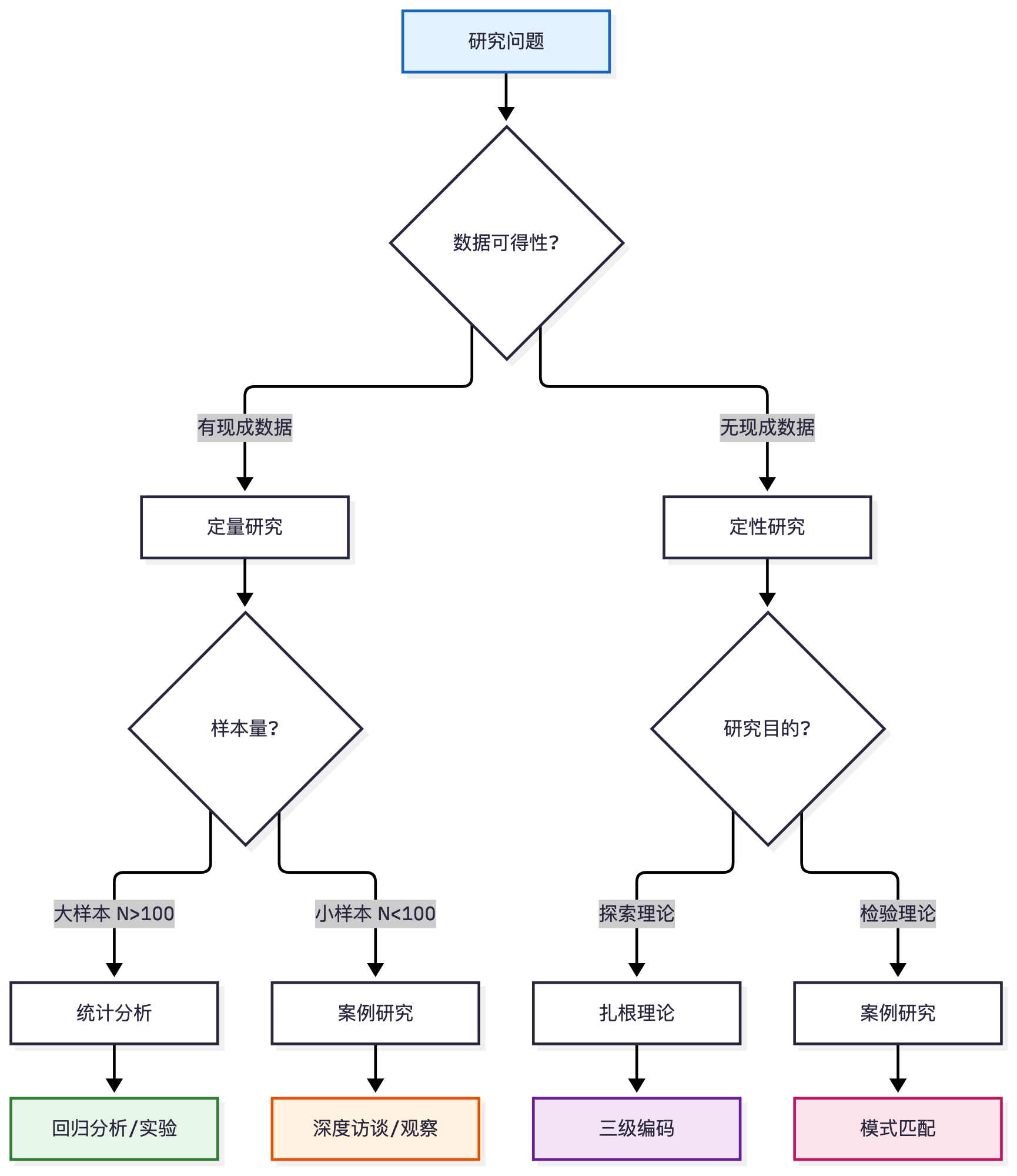
图 4.2 相关 ≠ 因果——三个金融故事的隐喻合图:遗漏变量 / 反向因果 / 选择偏差。
三个故事的统一格式(背下来)
表 4.13 三个故事的统一格式(背下来)。
L4|L4|L4|L4
要素 & 故事 1 & 故事 2 & 故事 3
现象 & 素养高的人爱买基金 & 投保农户产量高 & 参训农民收入高
错误推断 & 素养 → 基金参与 & 保险 → 产量 & 培训 → 收入
真实原因 & 收入同时影响两者 & 产量高者更愿投保 & 有能力者才参加培训
问题类型 & 遗漏变量 & 反向因果 & 选择偏差
首选解法 & FE / IV & 滞后变量 / FE / IV & RCT / DID / PSM
对应章节 & §9.2 / §9.3 & §9.1 / §9.2 / §9.3 & §9.4 / §9.5\
[提示] 答辩万能句:当被问“你怎么保证是 X→Y,而不是 Y→X,也不是第三个变量”,标准回答结构是——
“① 我承认存在这种可能;② 我用了 ___ 策略来缓解(并说明为什么这个策略能处理这一类偏误);③ 我做了 ___ 稳健性检验;④ 本文结论的因果强度限定为 ___(例如‘提供了与因果解释一致的证据’,而不是‘证明了因果’)。”
最糟糕的回答是“我的回归很显著,所以就是因果”。显著性只说明相关不太可能是抽样误差造成的,与因果毫无关系。
§4.5 研究策略三分选型
确定了问题类型、认清了效度威胁,下一步是选路线。本手册把经济研究的可行路线分成三条:
表 4.14 研究策略三分选型。
L5|L5|L5|L5|L5
路线 & 核心逻辑 & 数据形态 & 适用问题 & 手册章节
实证回归路线 & 大样本 + 统计识别 → 检验假说 & 面板 / 截面 / 市场数据(数值型) & 因果型、相关型(有明确变量和假说) & 第 9 章
案例研究路线 & 小样本 + 过程追踪 → 理解机制或构建理论 & 访谈 / 档案 / 观察(文本为主) & 描述型、How 型(机制不明、理论缺失) & 第 10 章
仿真实验路线 & 建 Agent 规则 + 计算机模拟 → 探索无法观测的系统 & 校准参数 + 模拟输出 & 系统层面、政策反事实、数据不可得 & 第 9 章 §9.8(选修)\
路线一:实证回归(经济研究的主流)
什么时候选:
你的假说可以写成“X 每增加 1 单位,Y 变化 β 单位”
你有几百个以上观测(或几十个以上个体 × 多期)
变量可以量化,数据已经或即将到手
要求:计量功底(第 9 章全套)+ 数据清洗能力(第 8 章)+ 稳健性检验意识(S9.1—S9.4)
典型产出:描述统计表 + 基准回归表 + 内生性处理表 + 稳健性表 + 机制检验表
路线二:案例研究(被严重低估的路线)
什么时候选:
研究问题还不太清楚,需要先弄清现象的性质和范围 → 探索性研究
现象很新,没有现成理论可以演绎 → 理论构建(归纳)
你想知道“过程是怎么发生的”,而不只是“效应有多大” → 机制追问
要求:访谈技巧 + 编码能力(第 10 章)+ 案例选择逻辑 + 多案例比较(提高可推广性)
△ 常见误解:“案例研究比较简单,因为不用跑回归。”恰恰相反——好的案例研究对理论敏感度、访谈质量、编码严谨性的要求极高。案例研究的优势是“能发掘出与未知现象相关的各种社会、文化和政治因素”,劣势是“对调查结果的解释可能取决于研究人员的观测和综合能力”,且单个案例的结论难以推广——多案例比较是主要的补救办法。
专硕特别提示:金融专硕(MF)和农村金融专硕的学位论文中,案例分析类是主流体裁之一。四类体裁(产品设计 / 解决方案 / 案例分析 / 调研报告)的骨架见附录 F——它们的“方案设计”章,本质上就是本章 research_design.md 的应用文版本。
路线三:仿真实验(ABM,选修)
什么时候选:
你关心的是系统层面的涌现结果,而不是单个个体的行为(例如:保险市场会不会崩溃?挤兑会不会传染?)
现实中无法做实验(你不能真的让一家银行倒闭看看后果)
你想做反事实政策模拟(如果补贴率从 30% 提到 50%,参保率会怎么变?)
要求:编程能力(Python / Mesa)+ 参数校准(用真实数据标定)+ 敏感性分析 + 对“仿真不是证据”的清醒认识
典型例子:四川水稻气象保险 ABM(川农团队实践)——用农户 Agent 模拟参保决策,检验不同补贴方案的覆盖率与财政成本。
△ 诚实边界:ABM 的结论依赖你设定的规则。规则错了,仿真再漂亮也是错的。所以 ABM 论文必须做敏感性分析,并明确说明“本文结论在何种假设下成立”。
选型决策:三个维度交叉
维度 1 · 数据形态
   有数值型大样本          -> 实证回归
   只有文本 / 访谈 / 档案   -> 案例研究
   两者都没有,但有可靠的机制假设 -> 仿真(且需真实数据校准)

维度 2 · 问题类型
   因果型(X->Y 有多大)    -> 实证回归
   How 型(过程 / 机制)    -> 案例研究(或实证 + 机制检验 §9.7)
   系统型(涌现 / 反事实)  -> 仿真

维度 3 · 理论成熟度
   理论成熟、有可检验假说   -> 实证回归(演绎)
   理论缺失、需从现象归纳   -> 案例研究(归纳)
   理论清晰但无法实证       -> 仿真
混合路线(推荐了解)
混合方法的价值——即使是结构化问卷,也可以加开放性问题收集定性数据。经济研究里常见的混合形态:
表 4.15 混合路线(推荐了解)。
L3|L3|L3
混合形态 & 做法 & 例子
先案例后实证 & 用访谈发现机制 → 用大样本检验 & 先访谈 20 户农户了解“为什么不愿投保” → 再用问卷数据检验这些原因
先实证后案例 & 回归发现异常或异质性 → 用案例解释 & 回归发现某类地区效应为负 → 实地调查解释为什么
实证 + 仿真 & 实证估计参数 → 仿真做政策推演 & 用调查数据校准 Agent 参数 → 模拟不同补贴方案的效果\
把选择写进方案
research_design.md 第五栏“方法路线”必须明确写出四件事:
我选的是哪条路线,为什么(对照上面三个维度)
我的设计属于三大类型的哪一类(真实验 / 准实验 / 非实验)
我预判的主要效度威胁是哪 1-2 条,打算怎么缓解
我放弃了什么(诚实说明局限)
§4.6 research_design.md 五栏模板
第 2 章你写了 research_question.md(现象 + 问题 + 构念),第 3 章升级为 one_page_proposal.md(八栏一页纸)。本章再升级为五栏完整方案。
为什么是“五栏”
一份研究计划应说明:研究问题、为什么选这个问题、有关这方面的已有知识、支持待检验假设的理论、怎样衡量构念、选择哪种研究方法、为什么选这个方法、所选择的抽样方法。压缩到硕士论文可操作的程度,就是五栏:
表 4.16 为什么是“五栏”。
L4|L4|L4|L4
栏 & 内容 & 回答的问题 & 前置章节
1 & 研究问题(精确化) & 到底问什么?什么类型? & 第 2、3 章
2 & 理论框架 & 凭什么这么问?构念怎么连? & 第 2 章 §2.4 + 本章框架图
3 & 研究假说 & 可检验的具体预测是什么? & 第 2 章 §2.3
4 & 数据方案 & 数据从哪来?变量怎么测? & 第 5、6 章
5 & 方法路线 & 怎么识别?怎么稳健? & 第 8、9 章\
完整模板(复制到你自己的 research_design.md)
# 研究设计方案(Research Design)

**姓名**:____ **方向**:[ ]农金 [ ]风险/保险 [ ]金融理论
**版本**:v1.0(第 4 章产出) **日期**:____
**上游文件**:research_question.md(第 2 章)、one_page_proposal.md(第 3 章)
**AI 使用声明(开题版)**:见文末附表(第 11 章 S11.1 要求,现在就开始写)

---

## 栏 1 · 研究问题(精确化)

### 1.1 从现象到问题

- 上游文件:research_question.md(第 2 章)、one_page_proposal.md(第 3 章)
- 现象描述(一句话):____
  例:数字金融试点政策在部分县域推行后,当地农户的信贷可得性似乎有所提高。
- 研究问题(一句话,含核心变量与情境):____
  例:数字金融试点政策是否提高了试点县农户的信贷可得性?
- 问题类型(打 √):
  [ ] 探索型(What is going on?)
  [ ] 描述型(How much / How many?)
  [ ] 因果型(Does X cause Y?)

### 1.2 问题细化——PICO 格式

| 要素 | 本研究的定义 | 填写 |
|------|-------------|------|
| P(Population) | 目标总体 | ____ |
| I(Intervention / Exposure) | 核心自变量 X | ____ |
| C(Comparison) | 对照 / 反事实 | ____ |
| O(Outcome) | 因变量 Y | ____ |

例:P = 中西部县域农户;I = 所在县被选为数字金融试点;
   C = 申报但未获批的邻近县农户;O = 农户新增贷款金额(元)。

### 1.3 文献缺口(Gap)定位

- 已有研究告诉了我们什么(3—5 条关键发现):
  1. ____
  2. ____
  3. ____
- 尚未回答的问题(Gap):____
- Gap 类型:
  [ ] 情境缺口(中国 / 农村场景尚无证据)
  [ ] 方法缺口(既有研究识别策略不够严格)
  [ ] 变量缺口(某个关键构念从未被测量)
  [ ] 理论缺口(现有理论无法解释新现象)
- Gap 强度自评:__/5(< 3 分建议换题——第 3 章 S3.2)

---

## 栏 2 · 理论框架

### 2.1 核论文论锚定

- 锚定论文 1(理论来源):作者(年份),核心观点:____
- 锚定论文 2(情境适配):作者(年份),核心观点:____
- (可选)锚定论文 3:作者(年份),核心观点:____

### 2.2 构念与逻辑链

用一段话或一张图说明"凭什么这么问"——构念之间的逻辑连接:

    [构念 A] ──(+)──> [构念 B] ──(+)──> [构念 C(Y)]
                          ↑
                     [调节变量 M]

- 主效应逻辑(A → Y 为什么成立?理论机制是什么?):
  ____
- 如果存在中介 / 机制变量,请说明传导渠道:
  ____
- 如果存在调节变量,请说明边界条件:
  ____

### 2.3 理论框架图

- [ ] 已画 theory_framework.png(可用 PPT / draw.io / TikZ)
- [ ] 图中每条箭头都标注了方向预期(+ / −)
- [ ] 图中每个构念都对应了栏 4 的测量方案

> 提示:画图不是装饰,是思维工具。画不出来的地方,
> 往往就是你没想清楚的地方。

---

## 栏 3 · 研究假说

### 3.1 假说清单

| 编号 | 假说内容 | 理论依据(哪篇文献 + 页码) | 对应变量 |
|------|---------|---------------------------|---------|
| H1 | ____ | 作者(年份),p.__ | X → Y |
| H2 | ____ | 作者(年份),p.__ | M → Y(机制) |
| H3 | ____ | 作者(年份),p.__ | 调节效应 |

### 3.2 假说推导自检

逐条检查(每条打 √ 或 ×):

- [ ] 每条假说都有至少 1 篇锚定文献支撑(不是你自己拍脑袋)
- [ ] 假说方向明确(写了"正向影响"而非"有影响")
- [ ] 假说可证伪(能用数据拒绝)
- [ ] 假说之间不矛盾(H1 和 H2 不互斥,除非你打算做竞争假说)
- [ ] 假说数量合理(硕士论文通常 2—4 条,超过 5 条需与导师商议)

### 3.3 竞争性假说(可选但加分)

- 是否存在与 H1 方向相反的竞争性解释?
  ____
- 你打算用什么数据 / 检验来区分两者?
  ____

---

## 栏 4 · 数据方案

### 4.1 数据来源

| 数据类别 | 具体来源 | 获取方式 | 时间范围 |
|---------|---------|---------|---------|
| 因变量 Y | ____ | ____ | ____ |
| 自变量 X | ____ | ____ | ____ |
| 控制变量 | ____ | ____ | ____ |
| 工具变量(如有) | ____ | ____ | ____ |

例:
| 数据类别 | 具体来源 | 获取方式 | 时间范围 |
|---------|---------|---------|---------|
| Y:农户信贷可得性 | CHFS 2019/2021 | 官网申请 | 2019—2021 |
| X:数字金融发展 | 北大数字普惠金融指数 | 公开下载 | 2011—2021 |
| 控制变量 | 县级统计年鉴 |  EPS / CEIC | 2011—2021 |

### 4.2 变量操作化

| 构念 | 变量名 | 测量方式 | 单位 | 数据来源 |
|------|-------|---------|------|---------|
| Y:信贷可得性 | loan_access | 过去 12 个月是否获得正规贷款 | 0/1 | CHFS |
| X:数字金融 | dig_finance | 北大数字普惠金融指数(县级) | 指数值 | 北大课题组 |
| 控制:经济发展 | pgdp | 人均 GDP(对数) | 万元(对数) | 统计年鉴 |
| 控制:产业结构 | industry | 第二产业增加值占 GDP 比重 | % | 统计年鉴 |
| 控制:财政依赖 | fiscal | 财政支出 / 财政收入 | 比值 | 统计年鉴 |

### 4.3 样本方案

- 分析单位(个体 / 家庭 / 企业 / 县 / 银行):____
- 抽样方法(随机 / 分层 / 方便 / 全样本):____
- 样本量预估:____
- 样本筛选条件(排除规则):
  1. ____
  2. ____
- 时间窗口:____ 至 ____

### 4.4 数据质量预评估

- [ ] 核心变量的缺失率已确认 < 20%(或已计划插补方案)
- [ ] 变量的变异系数合理(不是几乎全为 0 或全为 1)
- [ ] 数据时间跨度足以支撑因果推断(X 在 Y 之前)
- [ ] 已确认数据使用许可(版权 / 申请流程 / 费用)

---

## 栏 5 · 方法路线

### 5.1 路线选择与理由

- 我选的路线(打 √):
  [ ] 实证回归路线(第 9 章)
  [ ] 案例研究路线(第 10 章)
  [ ] 仿真实验路线(第 9 章 §9.8,选修)
  [ ] 混合路线:____ + ____

- 选择理由(对照 §4.5 三个维度):
  - 数据形态:____(数值型大样本 / 文本访谈 / 校准参数)
  - 问题类型:____(因果型 / How 型 / 系统型)
  - 理论成熟度:____(成熟可检验 / 缺失需归纳 / 清晰但无法实证)

### 5.2 设计类型

- 我的设计属于(打 √):
  [ ] 真实验(RCT)
  [ ] 准实验(DID / RDD / 政策评估)
  [ ] 非实验—事后追溯(面板 FE / 截面回归 / OLS)

- 判断依据(回顾 §4.3 自测流程图):
  ____

### 5.3 识别策略(核心!)

| 内生性来源 | 我的处理策略 | 对应章节 |
|-----------|-------------|---------|
| 遗漏变量 | ____ | §9.2(FE)/ §9.3(IV) |
| 反向因果 | ____ | §9.1(滞后变量)/ §9.2(FE) |
| 选择偏差 | ____ | §9.4(DID)/ §9.5(PSM) |
| 测量误差 | ____ | §9.3(IV)/ §9.6(稳健标准误) |

例(农金方向 DID 设计):
| 内生性来源 | 我的处理策略 | 对应章节 |
|-----------|-------------|---------|
| 遗漏变量 | 省份 + 年份双向 FE 吸收不随时间变的县特征和全国性冲击 | §9.2 |
| 选择偏差 | 试点县非随机挑选 → PSM-DID(先用可观测特征匹配再估计) | §9.5 |
| 同期政策干扰 | 加入"同期其他政策"控制变量 + 安慰剂检验(假装政策提前 2 年) | §9.4 |

### 5.4 基准模型设定

写出你的回归方程(用 LaTeX 或文字均可):

    Y_it = β₀ + β₁ X_it + γ Controls_it + μ_i + λ_t + ε_it

- 其中:i = ____(个体 / 县 / 银行),t = ____(年份 / 季度)
- β₁ 的含义:____
- 预期符号:β₁ > 0 / β₁ < 0(与 H1 对应)
- 聚类标准误层级:____(通常选"个体"或"地区")

### 5.5 稳健性检验计划(至少列 3 项)

| 编号 | 检验内容 | 目的 |
|------|---------|------|
| R1 | 替换核心变量测量方式 | 排除测量敏感性 |
| R2 | 缩尾处理 / 剔除极端值 | 排除异常值驱动 |
| R3 | 子样本回归(分东 / 中 / 西部) | 异质性分析 |
| R4 | 安慰剂检验(虚构处理时点) | 排除趋势性混淆 |
| R5 | 替换估计方法(如 OLS → Probit) | 排除模型设定依赖 |
| 补充 | ____ | ____ |

### 5.6 局限性(诚实声明)

- 本研究无法解决的问题:
  1. ____
  2. ____
- 结论的因果强度限定为:
  [ ] 因果效应估计(有外生变异支撑)
  [ ] 与因果解释一致的证据(识别策略有残余威胁)
  [ ] 相关关系描述(无因果声称)

---

## 效度威胁自查表(栏 5 配套)

写完五栏后,逐条检查七大效度威胁(回顾 §4.2):

| 威胁类型 | 是否可能 | 在本研究中的具体形式 | 现有缓解措施 | 补充策略 |
|---------|---------|-------------------|-------------|---------|
| 历史 | | | | |
| 成熟 | | | | |
| 测验效应 | | | | |
| 仪器变化 | | | | |
| 统计回归 | | | | |
| 选择偏差 | | | | |
| 样本流失 | | | | |
| | 效度威胁自查 | | 逐条判断是否成立 |

(这张表现在看着多余,第 11 章写 AI 使用声明时你会感谢自己——S11.1)
五栏与四类专硕体裁的对应(附录 F 预告)
表 4.17 五栏与四类专硕体裁的对应(附录 F 预告)。
L5|L5|L5|L5|L5
五栏 & 调研报告 & 案例分析 & 产品设计 & 解决方案
1 问题 & 调研背景与问题 & 案例企业面临的问题 & 产品需求分析 & 问题诊断
2 理论 & 理论依据(可简化) & 理论视角 & 设计原理 & 政策 / 理论依据
3 假说 & 调研假设 / 待验证问题 & 分析命题 & 产品功能假设 & 方案预期效果
4 数据 & 调查方案设计 & 案例资料来源 & 市场数据 / 客户数据 & 现状数据
5 方法 & 统计分析方法 & 案例比较逻辑 & 定价 / 风控模型 & 实施路径与评估\
[重点] 也就是说:同一份五栏方案,换一套标题就能变成四类体裁中任意一类的骨架。这就是“研究设计能力”的可迁移性——也是本手册希望专硕同学重点带走的东西。
🛠 AI 辅助研究栏|用法一:AI 辅助效度威胁自查(本章主打)
场景:你写完了五栏方案,但不知道自己漏了什么。这是 AI 最有价值也最安全的用法之一——因为它做的是“提出问题”,不是“给出结论”。
提示词模板:
最后那句“不要鼓励性评价”很关键——不写的话,AI 会先夸你三段,再轻描淡写地提两个无关痛痒的问题。
AI 输出示例(节选,农金方向):
表 4.18 威胁 / 是否可能 / 具体形式 / 现有缓解速查表。
L6|L6|L6|L6|L6|L6
威胁 & 是否可能 & 具体形式 & 现有缓解 & 补充策略 & 严重度
历史 & 是 & 2020—2022 年你的样本县同时经历脱贫攻坚收官与疫情,两项冲击与数字金融试点期重叠 & DID 对照组可吸收共同冲击 & 加“同期其他政策”控制变量;做安慰剂检验(假装政策提前两年) & 高
选择偏差 & 是 & 试点县由省里挑选,基础条件更好 & 无 & PSM 先匹配再 DID;或用“申报但未获批县”作对照 & 高
仪器变化 & 是 & 数字普惠金融指数 2021 年调整过编制方法 & 无 & 检查指数在 2021 年是否有跳跃;考虑分时段估计 & 中
统计回归 & 否 & 你的样本是全部县,不是极端县 & — & — & 低
样本流失 & 不确定 & 县级面板一般不缺县,但可能有县改区导致口径变化 & 无 & 核对行政区划变更年份 & 低\
你的下一步(关键):
Step 1  逐条判断 AI 说的对不对——它是“提示”,不是“裁决”
        (AI 可能过度报警:把你的设计说得一无是处;
          也可能漏报:看不出你数据里的具体问题)

Step 2  对“确实存在”的威胁,去第 9 章找对应工具,
        写进栏 5 的识别策略表

Step 3  对“AI 误判”的威胁,在你的方案里写一句话说明为什么它不适用
        (这句话在答辩时非常有用——说明你想过了)

Step 4  把 AI 指出但你无法解决的问题,如实写进“局限性”一节
        (诚实的局限讨论 > 假装没有问题)
[提示] 为什么这个用法安全:AI 在这里不产生任何“事实性内容”(不产生数据、不产生文献、不产生结论),只产生问题清单。问题错了最多浪费你几分钟,不会污染你的研究。这与“让 AI 写综述”(可能引入虚构文献,S3.1)有本质区别。
用法二:AI 辅助假说推导(注意 S4.1 边界)
场景:你有理论框架图,但不知道怎么把它拆成可检验的假说。
提示词模板:
第 ③④ 条是 S4.1 的技术化落实——通过提示词约束,让 AI 不去做它最容易犯错的事(编文献)。
△ 红线提醒:即使你在提示词里写了“不要编造文献”,AI 仍可能编。输出里出现的每一个“作者 年份”,都要用 Zotero 核实:
cli-anything-zotero add doi {DOI}                              # 有 DOI 就直接抓
cli-anything-zotero item semantic-search --query "作者 关键词"   # 在本地库里查
用法三:AI 辅助“研究问题精确化”
场景:你的问题还是“数字金融对农户收入的影响”这种宽泛表述,需要收窄到可做的程度。
提示词模板:
最后那句约束很重要:否则 AI 会建议你“做一个全国性的随机对照试验”——听起来很对,但你做不到。
本章 AI 用法总纲
表 4.19 本章 AI 用法总纲。
L4|L4|L4|L4
用法 & AI 的角色 & 你的角色 & 风险等级
效度威胁自查 & 提出问题清单 & 逐条判断成立与否 & • 低
假说推导 & 按你给的框架拆解成可检验形式 & 逐条核实文献、判断理论逻辑 & • 中(S4.1)
问题精确化 & 指出过宽之处 & 决定收窄方向 & • 低
~~直接生成理论框架~~ & — & — & • 禁止(S2.1 / S4.1)
~~直接生成文献综述~~ & — & — & • 禁止(S3.1 / S3.2)\
🛡 AI 诚信栏|S4.1 假说必有文献支撑
红线:research_design.md 栏 3 的每一条假说,必须指向至少 1 篇真实存在的已发表论文或教材章节。没有文献支撑的假说不是假说,是猜测。
这条红线管什么
表 4.20 情形 / 判定速查表。
L2|L2
情形 & 判定
写“根据金融排斥理论,数字金融可得性提高农户收入”,且能指出相关经典与实证文献确实支持这一推论 & ✅ 合规
写“根据 XX 理论”,但你查 XX 理论原文,发现它并不支持你这个推论 & ❌ 不端——这是“理论误引”,比不引用更严重
AI 说“Lusardi & Mitchell(2014)发现金融素养提高投资回报率”,你直接写进假说依据,但没查原文 & ❌ 高危——该文献可能不存在,或存在但没有这个结论
你的假说是自己的原创推测,并明确标注“本文提出,尚无直接文献支撑,属探索性假说” & ✅ 合规(诚实标注即可)\
为什么“理论误引”特别严重
因为它具有欺骗性:格式规范、文献真实、逻辑通顺,只有读过原文的人才知道你把作者的观点说反了或说过头了。而审稿人恰好就是那个人。
常见的三种误引:
过度外推:原文说“在发展中国家样本中相关”,你写成“具有普遍因果效应”
张冠李戴:原文说的是 A 对 B 的影响,你引它来支持 A 对 C 的影响
反向引用:原文其实在质疑这个关系,你引它来支持这个关系
检查方法(每条假说四步)
Step 1 · 定位
   打开你引的那篇文献,找到支撑该假说的**具体段落**(记下页码)

Step 2 · 核对方向
   原文的结论方向(正 / 负 / 不显著)与你的假说方向一致吗?

Step 3 · 核对边界
   原文的样本、情境、条件与你的研究可比吗?
   如果原文是“美国上市公司”,你是“中国小农户”——
   你需要额外论证为什么可以外推。
   (这个论证本身可能就是你的贡献点)

Step 4 · 记录
   在 research_design.md 栏 3 的表格里,把“作者 年份 + 页码”写进去。
   写不出页码 = 你没真读过 = 回到 Step 1
开题前自查表(逐条打勾)
表 4.21 检查项 / 状态速查表。
L2|L2
检查项 & 状态
栏 3 每条假说都有至少 1 个“作者 年份”支撑 & ☐
每条支撑文献都已用 Zotero 核实存在(DOI 解析通过) & ☐
每条支撑文献我都定位到了具体页码 / 章节 & ☐
没有任何一条是“AI 说有但我没查到原文”的 & ☐
原文结论方向与我的假说方向一致(无过度外推) & ☐
原文情境与我的研究情境可比,或我已论证可比性 & ☐
探索性假说(无文献支撑的)已明确标注 & ☐
理论框架图 theory_framework.png 每条箭头都有文献标注 & ☐\
和第 2 章 S2.1 的关系:S2.1 管“理论框架图的每条箭头”,S4.1 管“每条假说”。箭头是假说的图形化表达,两者必须一致——图上有的箭头,栏 3 里要有对应假说;栏 3 里的假说,图上要能找到对应箭头。开题时导师常做的第一件事,就是把这两样对照着看。
AI 使用声明(本章版本)
在 research_design.md 末尾附上。第 11 章 S11.1 会要求三个版本(开题 / 投稿 / 答辩),现在就从开题版开始记:
## AI 使用声明(开题版)

本研究方案撰写过程中使用了生成式 AI 辅助,具体如下:

| 环节 | 用途 | 工具 | 人工核对方式 | AI 是否产出最终内容 |
|---|---|---|---|---|
| 文献梳理 | 从 30 篇摘要中抽取概念矩阵字段 | ____ | 逐格对照原文核对 | 否 |
| 理论框架 | 生成 mermaid 初稿 | ____ | 逐箭头核实文献支撑 | 否 |
| 假说推导 | 按已定框架拆解为可检验形式 | ____ | 逐条核实文献 + 判断理论逻辑 | 否 |
| 效度自查 | 按七大威胁提出问题清单 | ____ | 逐条判断是否成立 | 否 |
| 文字表达 | ____ | ____ | ____ | ____ |

**声明**:所有假说、理论关系、文献引用均经本人核实;研究设计的判断与决策由本人
独立作出;本文不包含任何由 AI 生成而未经核实的事实性内容。

签名:____  日期:____
△ 这张表必须真实。写了“逐格核对”却其实没核对,比不写声明更严重——那是虚假陈述,违反第 0 章 §0.4 研究道德四准则中的“诚实”。
English Edition
Chapter 4 · Research Design
Learning Objectives
After completing this chapter, you should be able to:
State the seven threats to internal validity (history / maturation / testing / instrumentation / statistical regression / selection / attrition), with one finance example each
Distinguish the three design types (true experiment / quasi-experiment / non-experimental—ex post facto) and classify your own study
Explain omitted variables, reverse causality, and selection bias via three finance stories of “correlation ≠ causation”
Write the five-field
research_design.mdplan (question / theory / hypotheses / data / method)
[Takeaway] This chapter is short, but it is the handbook’s “load-bearing wall.” Every identification strategy in Chapter 9 (IV / DID / PSM / RDD / FE) is essentially answering the one question this chapter poses: on what grounds do you claim X causes Y?
§4.1 Three Types of Research Questions
📐 结构图示(书版示意图的文字要点)
- tikzpicture
- ->,very thick,NavyBlue
- Exploratory
- What is going on?
- E.g.:
- Methods:
- Sample:
- Output:
Figure 4.1 Three types of research question—not parallel options but three progressive layers: map the phenomenon, quantify it, then identify causation.
Three Progressive Layers, Not Three Parallel Options
Descriptive   ->   Correlational   ->   Causal
(know what exists)(know it is related)(know who causes whom)

   evidence strength ^     method difficulty ^     data demand ^     workload ^
Discuss causation without description, and readers do not know what your sample looks like
Discuss causation without correlation, and you do not even know whether it is “worth digging into”
But stopping at description and correlation cannot publish in good journals—reviewers will ask “So what?”
Type Determines Method
Table 4.1 Type determines method.
L3|L3|L3
Your question type & Minimum method requirement & Handbook chapters
Descriptive & Representative sample + normative statistical reporting + a sound indicator system & Ch. 5 (sampling) + Ch. 8 (descriptive statistics)
Correlational & Regression + controls + significance testing & Ch. 9 §9.1 (OLS)
Causal & Identification strategy + endogeneity discussion + robustness + mechanism tests & Ch. 9 §9.2–9.7 in full\
△ The most common fatal error: writing a causal question (“the effect of digital finance on farm income”) while using a correlational method (running one OLS and calling it done). Advisors bounce this at the proposal stage; journals reject it outright at submission.
Two ways out—pick one:
Downgrade the question: change “effect” to “association”—honest and easy, but the contribution shrinks
Upgrade the method: find an identification strategy (policy shock → DID; exogenous instrument → IV; participation threshold → RDD)—harder, but this is the publishable road
[Takeaway] Internal validity is causation, and it requires three conditions—① cause and outcome are associated; ② temporal precedence (cause precedes effect); ③ no other plausible explanation (no spuriousness). Every method in Chapter 9 works hard to satisfy ② and ③.
Three-Track Exercise
Take the research question in your Chapter 3 one_page_proposal.md and write it once per type:
Table 4.2 Three-track exercise.
L4|L4|L4|L4
Track & Descriptive version & Correlational version & Causal version
【Agri】 rural finance & Current status and distribution of farm households’ digital finance use in Sichuan Province & Is digital finance use correlated with farm income & Does digital finance use raise farm income (identification: ___)
【Ins】 risk management/insurance & Coverage and claims of the full-cost insurance pilot for the three staple grains & Is agricultural insurance participation correlated with farm production investment & Did the full-cost insurance pilot raise grain output (identification: DID)
【Fin】 finance theory & policy & Distributional changes in lending rates after the LPR reform & Are LPR changes correlated with corporate investment & Did LPR cuts stimulate corporate investment via the credit channel (identification: ___)\
Then ask yourself two questions: which layer do I intend to do? Am I able to do that layer?
§4.2 Internal and External Validity: The Seven Threats
Two Kinds of Validity First
Table 4.3 Two kinds of validity first.
L4|L4|L4|L4
Validity & Asks & Plain words & Standard definition
Internal validity & Did X really cause Y? & “Did it do it?” & Whether changes in the dependent variable are indeed caused by the presumed independent variable, not by extraneous variables
External validity & Does the conclusion generalize? & “Does it hold elsewhere, for others?” & Whether observed associations generalize from sample to population (population validity), or hold for other people / organizations / settings / times (ecological validity)\
[Key point] Two more kinds of validity: construct validity (does your scale really measure that construct?) and statistical conclusion validity (is the statistical method right, are its assumptions satisfied?). These are covered in Chapters 5 and 9 respectively.
The trade-off: internal and external validity often trade off—laboratory experiments are high on internal but low on external validity (artificial settings misrepresent the real world); field surveys are high on external but low on internal validity (you cannot manipulate the independent variable). The overwhelming majority of economic research sits on the “higher external, lower internal” side of this trade-off—which is exactly why identification strategies are needed.
Reviewing the 2021 Nobel Memorial Prize (Angrist, Imbens, Card), Li Baoliang and Guo Qiyou[78] note that the core of econometrics’ “credibility revolution” is: the credibility of causal evaluation depends not on data or econometric methods themselves, but on a deep understanding of the institutional processes behind the natural experiment. In other words, good identification strategies come from institutional knowledge, not technical tools—only by deeply understanding the selection mechanism of agricultural insurance pilots can you find a valid DID discontinuity; only by understanding a digital finance platform’s entry thresholds can you find a natural cutoff for RDD. This echoes the “competence circle” question of §3.7: competence is not merely “can I run DID/Stata” but “do I understand how this policy/institution works.” Beginners often learn IV/DID first and then hunt for a topic—the correct order is the reverse: deep institutional understanding first, and the identification strategy follows naturally.
The Seven Threats to Internal Validity
Table 4.4 The seven threats to internal validity.
L4|L4|L4|L4
# & Threat & Meaning & Example
1 & History & The observed outcome was caused by external events during the study period, not by the treatment & “Your study window happens to coincide with an LPR cut / the pandemic / property-market tightening”—outcomes changed, but not because of your X
2 & Maturation & The outcome reflects subjects’ natural development, not the treatment & “In the three-year panel, farmers learn and accumulate experience; financial literacy rises naturally”—no credit to the training
3 & Testing & The pretest affects the posttest (subjects remember answers or learn to cope) & “After being asked about income once, farmers learn to under-report (or remember the questionnaire)”—round-two data “improves”
4 & Instrumentation & Measurement tools or standards change between measurements & “The statistical caliber changed in 2020”; “the digital financial inclusion index methodology was revised in 2021”—data jumps that are not reality jumps
5 & Statistical regression (regression to the mean) & Extreme values regress toward the mean at second measurement & “You deliberately pilot in the poorest villages; next year they naturally improve”—not policy effectiveness, just mean reversion
6 & Selection & Treatment and control groups are inherently non-equivalent & “Insured farmers are all risk-averse types”; “pilot counties were hand-picked advanced counties anyway”
7 & Attrition & Subjects exit systematically, at different rates across groups & “In the three-year panel, 20% of farmers are lost to follow-up—mostly migrant workers, precisely those whose incomes changed most”\
The Three Most Commonly Tripped in Economic Research
① Selection Bias—Economic Research’s Killer No. 1
Any “voluntary participation” program has this problem: insurance, loans, training, cooperatives, digital wallets. Those who participate and those who do not differ from the start (risk preference, ability, wealth, social ties).
Observation: insured farmers' average output > uninsured farmers'
Wrong inference: agricultural insurance raises output
Likely truth: higher-output, income-stable farmers are wealthier and more
         motivated to insure (i.e., "output -> insuring", not "insuring -> output")
How to defend: random assignment (RCT, cleanest) / propensity score matching PSM (match on observables) / instrumental variables IV (find exogenous variation) / regression discontinuity RDD (exploit participation thresholds). → Ch. 9 §9.3, §9.5
② History—The Common Trap of Policy Evaluation
Observation: in 2020, pilot counties' farm income grew faster than non-pilot counties'
Wrong inference: the digital finance pilot worked
Likely truth: 2020 was also the final year of the poverty-alleviation campaign;
         pilot counties simultaneously received large other transfers
How to defend: DID (the control group absorbs common time shocks) + parallel-trends tests; control for concurrent policy variables; placebo tests (artificially advance the policy date and see whether the “effect” vanishes). → Ch. 9 §9.4
③ Statistical Regression—The Inevitable Price of “Picking the Worst Samples”
Poverty alleviation and inclusion programs naturally select “the most difficult samples.” Those extreme samples will most likely improve naturally next period—this is not policy effect; it is a statistical regularity.
Observation: after microcredit, the poorest 100 households' income rose 18% on average next year
Wrong inference: microcredit raised income by 18%
Likely truth: even without loans, many of these 100 would have rebounded naturally (mean reversion)
How to defend: build a control group screened by the same rule (the key is identical screening); use DID instead of simple before–after comparison.
External Validity: How Far Does Your Conclusion Travel?
Internal validity settles “did it do it”; external validity asks “does it do it elsewhere?” Three common generalization barriers:
Table 4.5 External validity: how far does your conclusion travel?
L3|L3|L3
Barrier & Finance example & Response
Sample representativeness & You surveyed 3 counties in the Chengdu plain—can you speak of “Sichuan,” let alone “China”? & Describe the sampling frame, report sample–population differences, carefully bound the conclusions
Setting specificity & China’s digital finance rides on extremely high mobile-payment penetration; India’s conclusions cannot be transplanted, nor vice versa & State the institutional background explicitly; discuss “boundary conditions”
Time specificity & Do financial-market behaviors during the 2020 pandemic generalize to normal times? & Add time dummies; run subsample robustness checks\
△ Honesty principle: insufficient external validity is not fatal; pretending it is high is. Writing “our conclusions carry important implications for national rural finance reform” on a sample of 300 households in one county—submission reviewers and thesis external examiners will see through it at a glance. Write instead: “Based on a survey of 300 households in XX county, generalization requires caution; future research should test further in… settings.”
§4.3 Three Design Types
Type 1: True Experiment
Definition: the researcher manipulates the independent variable (administers the treatment) and randomly assigns subjects to treatment and control groups.
Random assignment
   +-- Treatment group: receives treatment (e.g., digital finance training)
   +-- Control group: receives none (or a placebo)
        v after a period
   Compare the groups' dependent-variable difference -> the treatment effect
Why internal validity is highest: randomization equalizes the two groups in expectation on all dimensions—including unobservable ability, risk preference, and social ties. Selection, maturation, history, and statistical regression are all “averaged away.”
Rare in finance, but not absent:
RCTs in development economics / financial inclusion: randomly rolling out mobile payment in some villages, randomly allocating microcredit amounts or insurance subsidies—the methodological tradition established by the 2019 Nobel Memorial Prize (Banerjee, Duflo, Kremer)
Experimental economics / behavioral finance: laboratory subjects making investment decisions, risk-preference tasks, intertemporal choice tasks
Field experiments in corporate finance: randomly pushing an information-disclosure format to some investors and observing trading behavior
【Banerjee-School RCT Literature Support (GB/T 7714—2025)】
Table 4.6 Four representative works of the Banerjee-school RCT tradition—numbered to match the method-contribution notes below.
| No. | Authors·Year (GB/T 7714) | DOI (clickable) | Publisher online |
| 1 | BANERJEE A V, COLE S, DUFLO E, et al. Remedying education: evidence from two randomized experiments in India[J]. Quarterly Journal of Economics, 2007, 122(3): 1235–1264. | 10.1162/qjec.122.3.1235 | https://academic.oup.com/qje/article-abstract/122/3/1235/2504023 |
| 2 | BANERJEE A V, BANERJI R, BERRY J, et al. From proof of concept to scalable policies: challenges and solutions, with an application[J]. Journal of Economic Perspectives, 2017, 31(4): 73–102. | 10.1257/jep.31.4.73 | https://www.aeaweb.org/articles?id=10.1257/jep.31.4.73 |
| 3 | BANERJEE A V, DUFLO E. The experimental approach to development economics[J]. Annual Review of Economics, 2009, 1: 151–178. | 10.1146/annurev.economics.050708.143235 | https://www.annualreviews.org/doi/10.1146/annurev.economics.050708.143235 |
| 4 | DUFLO E, GLENNERSTER R, KREMER M. Using randomization in development economics research: a toolkit[M]//SCHULTZ T P, STRAUSS J. Handbook of Development Economics. Vol. 4. Amsterdam: Elsevier, 2007: 3895–3962. | 10.1016/S1573-4471(07)04061-2 | https://www.sciencedirect.com/science/article/pii/S1573447107040612 |
【Method Contributions at a Glance】
Banerjee et al. 2007 (QJE): Method contribution: using two replicated RCTs (half of schools randomly given extra teachers/computer-aided learning in Vadodara and Udaipur, India), shows “small classes + computer-aided learning” significantly improves marginal students’ math and language scores—the Banerjee/Duflo landmark in pushing RCTs from single-site pilots to cross-region replication. Implication for rural finance research: RCT designs for the same inclusion product across counties should build in replication logic, avoiding “works in one city, roll out nationally” over-extrapolation.
Banerjee et al. 2017 (JEP): Method contribution: proposes the three-stage model from “proof of concept to scalable policies”: ① multi-armed RCTs identify the most effective intervention in small samples; ② cluster randomization validates external validity at medium scale; ③ administrative data + rolling evaluation monitors drift at scale. Crucial when students design “rural digital credit RCTs”—stage-three implementation feasibility must be considered, or effects may decay by over 70% at scale.
Banerjee–Duflo 2009 (ARE): Method contribution: the authoritative survey of RCT methodology—argues systematically “why randomization is the optimal causal identification strategy in development economics” and compares RCT against IV/DID/RDD boundaries. Extremely valuable at the topic stage: prefer RCT when your intervention can be randomized and the sample suffices; otherwise fall back to quasi-experiments (the IV/DID/RDD/PSM paths below).
Duflo–Glennerster–Kremer 2007 (Handbook): Method contribution: the RCT operations manual—sample-size formulas (minimum detectable effect, MDE), balance-check tables, cluster-randomized designs, ITT vs ToT estimation and conversion, attrition handling, compliance checklists. Students wanting “randomly allocated microcredit amounts” as an empirical strategy should adopt this chapter’s experiment-design checklist directly, avoiding 80% of methodological rookie errors.
【Usage tips】: ① read Banerjee et al. 2007 for cross-region replication practice; ② read Banerjee et al. 2017 for the three stages from pilot to scale; ③ read Banerjee–Duflo 2009 to weigh RCT against Chapter 9’s IV/DID; ④ read Duflo–Glennerster–Kremer 2007 as a replicable checklist template—together the four form the complete evidence chain of the “Banerjee-school RCT tradition.”
【Supporting Pair: Experimental Economics / Behavioral Finance + Corporate Finance Field Experiments】
Table 4.7 Four representative works in behavioral finance and corporate finance field experiments—covering “experimental economics / behavioral finance” and “corporate finance field experiments” respectively.
| No. | Authors·Year (GB/T 7714) | DOI (clickable) | Publisher online |
| Experimental economics / behavioral finance (laboratory) | |||
| 5 | KAHNEMAN D, TVERSKY A. Prospect theory: an analysis of decision under risk[J]. Econometrica, 1979, 47(2): 263–292. | 10.2307/1914185 | https://www.jstor.org/stable/1914185 |
| 6 | FEHR E, GÄCHTER S. Fairness and retaliation: the economics of reciprocity[J]. Journal of Economic Perspectives, 2000, 14(3): 159–181. | 10.1257/jep.14.3.159 | https://www.aeaweb.org/articles?id=10.1257/jep.14.3.159 |
| Corporate finance field experiments | |||
| 7 | KARLAN D, ZINMAN J. Observing unobservables: identifying information asymmetries with a consumer credit field experiment[J]. Econometrica, 2009, 77(6): 1993–2008. | 10.3982/ECTA5781 | https://onlinelibrary.wiley.com/doi/abs/10.3982/ECTA5781 |
| 8 | DUFLO E, SAEZ E. The role of information and social interactions in retirement plan decisions: evidence from a randomized experiment[J]. Quarterly Journal of Economics, 2003, 118(3): 815–842. | 10.1162/00335530360698432 | https://academic.oup.com/qje/article-abstract/118/3/815/1943005 |
【Method Contributions at a Glance】
Kahneman–Tversky 1979 (Econometrica): Method contribution: the founding work of behavioral finance—prospect theory replaces the expected utility function with a value function (loss aversion + diminishing sensitivity) and a weighting function (nonlinear probability weighting), explaining endowment effects, loss aversion, probability neglect in real investment decisions; Kahneman won the 2022 Nobel Memorial Prize. Implication: any financial empirics assuming “rational agents” ignores real behavioral biases—“digital finance adoption” studies must include loss-aversion/anchoring behavioral variables.
Fehr–Gächter 2000 (JEP): Method contribution: using public goods games with punishment, shows people carry out altruistic punishment even in anonymous one-shot games, even when punishment is costly—challenging classical “rational self-interest” and founding the empirical basis of behavioral game theory. Implication for rural finance: cooperative finance / mutual aid sustainability cannot be modeled by rational agents alone; reputation, reciprocity, and social preferences must enter.
Karlan–Zinman 2009 (Econometrica): Method contribution: a South African consumer-credit field experiment (randomized credit offers) identifies adverse selection vs moral hazard—“rejected applicants default less ex post” ⇒ adverse selection exists; “those who accept high rates default more” ⇒ moral hazard exists—solving the identification problem of unobservable information asymmetry, the methodological template for inclusion-finance field experiments. Highly valuable for “rural microcredit effects” studies: randomized credit offers + ex-post default tracking is the standard operation for separating the two asymmetries.
Duflo–Saez 2003 (QJE): Method contribution: randomly gives employees retirement-savings information + colleagues’ social-network information on a university campus, showing information interventions + peer effects significantly raise retirement-plan participation; establishes the identification paradigm (information intervention + cluster randomization) for field experiments in corporate finance/employee benefits. Implication: investor behavior / governance mechanisms / disclosure effects in corporate finance can be identified by field experiments, not only OLS/DID.
【Usage tips】: ① read Kahneman–Tversky 1979 for the behavioral-finance foundation; ② read Fehr–Gächter 2000 for the behavioral-game paradigm; ③ read Karlan–Zinman 2009 for adverse-selection identification in inclusion finance; ④ read Duflo–Saez 2003 for randomized interventions on employee behavior—the four form the complete evidence chain of “behavioral finance + corporate field experiments”; combined with Table 4.6’s four, they cover all RCT application directions in economic research.
Difficulties: ① ethics (the control group is denied potential benefits); ② high cost and long cycles; ③ many financial variables simply cannot be randomized (you cannot randomize a county’s LPR).
Type 2: Quasi-Experiment
Definition: there is a “treatment” and a “comparison,” but assignment is not random. “A quasi-experimental design is almost identical to a true experimental design except in one respect: random assignment.”
Typical forms in finance:
Table 4.8 Type 2: quasi-experiment.
L3|L3|L3
Form & What the treatment is & Why it is not random
Policy-pilot evaluation (DID) & A county designated a digital-finance reform pilot zone & Pilot counties are selected by higher authorities, often with better fundamentals
Threshold effects (RDD) & Only those below an income line receive the subsidy & Assignment is determined by crossing a threshold on a continuous variable, not by lottery
Exogenous shocks & A natural disaster occurs / a regulation takes effect & Who is hit by the shock is beyond the researcher’s control
Matched comparison (PSM) & Participants vs similar non-participants & “Similar” holds only on observable dimensions\
【Quasi-Experimental Method Literature Support (GB/T 7714—2025)】
Table 4.9 Four classics of quasi-experimental methods—covering the core origins of DID, RDD, and PSM.
| No. | Authors·Year (GB/T 7714) | DOI (clickable) | Publisher online |
| Difference-in-differences (DID) | |||
| 1 | CARD D, KRUEGER A B. Minimum wages and employment: a case study of the fast-food industry in New Jersey and Pennsylvania[J]. American Economic Review, 1994, 84(4): 772–793. | 10.1257/000282806701157401 | https://www.jstor.org/stable/2118030 |
| 2 | BERTRAND M, DUFLO E, MULLAINATHAN S. How much should we trust differences-in-differences estimates?[J]. Quarterly Journal of Economics, 2004, 119(1): 249–275. | 10.1162/0033553041502244 | https://academic.oup.com/qje/article-abstract/119/1/249/1876068 |
| Regression discontinuity (RDD) | |||
| 3 | HAHN J, TODD P, VAN DER KLAAUW W. Identification and estimation of treatment effects with a regression-discontinuity design[J]. Econometrica, 2001, 69(1): 201–209. | 10.1111/0012-9682.00143 | https://www.jstor.org/stable/2692190 |
| Propensity score matching (PSM) | |||
| 4 | ROSENBAUM P R, RUBIN D B. The central role of the propensity score in observational studies for causal effects[J]. Biometrika, 1983, 70(1): 41–55. | 10.1093/biomet/70.1.41 | https://academic.oup.com/biomet/article-abstract/70/1/41/240879 |
【Method Contributions at a Glance】
Card–Krueger 1994 (AER): Method contribution: natural experiment + difference-in-differences—New Jersey raised its minimum wage from $4.25 to $5.05 in April 1992 while neighboring Pennsylvania did not; comparing fast-food employment across the two states finds no employment decline from the wage increase (if anything slightly positive), overturning classical “minimum wage → unemployment” theory; Card and Krueger won multiple awards for related work in 2006/2007. Implication: any setting with “a policy shock + treated/control groups” can host a DID—pilot-county evaluations of rural digital finance, inclusion-policy effects on county-level small firms’ credit access, deposit insurance’s effects on bank risk-taking.
Bertrand–Duflo–Mullainathan 2004 (QJE): Method contribution: Monte Carlo evidence that when DID outcomes are serially correlated (e.g., individual-level residual correlation), ordinary OLS standard errors are severely understated (a true 5% significance can masquerade as 0.1%); proposes clustering + collapsing + explicit modeling corrections, founding the methodology of DID standard-error adjustment (17,000+ citations). Warning for students: DID on individual-level panels requires individual fixed effects + standard errors clustered at the treatment level, or your significance may be a statistical illusion.
Hahn–Todd–Van der Klaauw 2001 (Econometrica): Method contribution: proves the identification theorem for sharp/fuzzy RDD—when the running variable crosses a known cutoff and the treatment probability jumps, treatment effects can be estimated without bias by local linear regression on either side; after 2001 RDD spread from electoral education studies to finance/labor/health evaluation. Implication: any financial policy with a “threshold rule” (differentiated bank regulation at capital-adequacy cutoffs, targeted RRR cuts for small banks, differentiated green-credit capital requirements by industry) can be an RDD—the two sides of the threshold are “naturally grouped” treatment and control.
Rosenbaum–Rubin 1983 (Biometrika): Method contribution: introduces the propensity score—the conditional probability of treatment given covariates
—and proves that conditioning on the propensity score makes treatment independent of potential outcomes, so matching/stratification/weighting on the score removes observed confounding; it founded causal inference for observational studies (47,000+ citations, among the most-cited papers in econometrics/statistics). Implication: for economic research that cannot be randomized and lacks clean policy shocks (small firms with vs without loans; digital finance adopters vs non-adopters), PSM is the cheapest identification scheme—but it balances only observables; unobserved confounding remains, so sensitivity analysis (Rosenbaum bounds) is mandatory.
【Supporting Pair: China’s Indigenous DID Application】
Table 4.10 A representative indigenous Chinese DID application—Zhou Li’an (2007) uses province-level panels + official turnover as a “natural experiment” to identify promotion incentives’ effect on growth.
| No. | Authors·Year (GB/T 7714) | DOI (clickable) | Publisher online |
| 5 | 周黎安. 中国地方官员的晋升锦标赛模式研究[J]. 经济研究, 2007(7): 36–50. | — | https://www.cnki.com.cn/Article/CJFDTotal-JJYJ200707003.htm |
【Method Contributions at a Glance】
- Zhou Li’an 2007 (Economic Research Journal): Method contribution: uses Chinese provincial panels + official turnover as exogenous shocks to argue systematically the link between local officials’ promotion and GDP growth—building the “promotion tournament” framework for China’s growth miracle; a landmark of political economy + quasi-experimental design in China (CSSCI-indexed, 3,900+ citations). Implication: Chinese financial policy evaluation has natural quasi-experimental soil—local governments’ behavioral differences, pilot counties’ non-random selection, staggered implementation timing are all natural treated/control opportunities; for “inclusion policy,” “digital finance pilots,” “green credit” evaluations, DID + two-way fixed effects (province + year) is the first choice.
【Usage tips】: ① read Card–Krueger 1994 for the birth case of DID in labor economics; ② read Bertrand et al. 2004 for DID standard-error adjustment (mandatory warning); ③ read Hahn et al. 2001 for the RDD identification theorem; ④ read Rosenbaum–Rubin 1983 for the founding of PSM; ⑤ read Zhou Li’an 2007 for DID in Chinese political economy—together the five form the complete evidence chain of the “quasi-experimental method tradition”; combined with Tables 4.6+4.7 (8 RCT papers), they cover all causal identification strategies in economic research.
The cost: there is a whole family of “selection-related threats”—selection–maturation, selection–history, selection–regression, selection–instrumentation, selection–testing, selection–attrition. Because the two groups are not equivalent to begin with, anything correlated with group membership can masquerade as a treatment effect.
Conclusion: a quasi-experiment’s internal validity is lower than a true experiment’s but higher than a purely observational study’s. Your paper must explicitly discuss which type your design is, which threats apply, and how you mitigate them—this is precisely the point of Chapter 9’s robustness checks.
Type 3: Non-Experimental—Ex Post Facto
Definition: the researcher manipulates nothing, only observes data already generated, using statistical methods to test relationships among variables.
This is the mainstream form of economic research, including:
Cross-sectional surveys: CHFS (China Household Finance Survey), CFPS (China Family Panel Studies), your own questionnaire
Panel data: county panels, listed-firm panels, bank-level panels
Market data: stock returns, bond prices, macro time series
Administrative and yearbook data: the People’s Bank of China, the financial regulator, the National Bureau of Statistics, FAO, IMF, World Bank
【Non-Experimental (Ex Post Facto) Method Literature Support (GB/T 7714—2025)】
Table 4.11 Four classics of non-experimental (ex post facto) methods—the first three are international panel-data methodology textbooks (Wooldridge / Baltagi / Hsiao), the fourth a Chinese advanced econometrics + Stata textbook.
【Method Contributions at a Glance】
Wooldridge 2010 (MIT Press, 2nd ed.): Method contribution: Econometric Analysis of Cross Section and Panel Data, 2nd edition—the bible of panel-data methodology, systematically covering the identification conditions and asymptotic properties of cross-sectional OLS / IV / fixed effects / random effects / dynamic panels / discrete-choice panels / censored panels / random-effects Probit, with Stata practice commands (72,000+ citations, the most-cited of all panel-data methodology references). Core value for students: county/province/firm-level fixed effects, clustered standard errors, heteroskedasticity-robust errors, Hausman tests, and Wooldridge-style panel robustness checks are all in this book—mandatory reading for “Chinese county-panel” research.
Baltagi 2005 (Wiley, 3rd ed.): Method contribution: the companion classic to Wooldridge—more modular, easy for looking up a particular estimator’s properties; the Arellano–Bond / Blundell–Bond GMM derivations of dynamic panels are clear, the standard toolkit for “macro + micro dynamics” trade-offs. Directly helpful for “official turnover → growth” or “bank executive turnover → risk-taking” studies.
Hsiao 2003 (Cambridge, 2nd ed.): Method contribution: the early authority of panel-data methodology, with the deepest coverage of dynamic panels, panel unit roots, panel cointegration, and spatial panels—used in economic research for mixed time-series-panel data such as interest rates / exchange rates / money supply. Econometric Society Monograph No. 34, an authoritative recommendation of the Econometric Society.
Chen Qiang 2014 (Higher Education Press, 2nd ed.): Method contribution: one of China’s most authoritative advanced econometrics textbooks—every method comes with Stata commands and Chinese annotations, covering cross-section / panel / time series / VAR / GMM / discrete choice / quantile regression; the standard textbook of Chinese economics master’s and PhD econometrics courses, and the practical guide for research on CHFS / CLDS / CGSS microdata. Core value for students: the first book to open when Stata throws an error on Chinese financial empirics—it has a complete method-command-example mapping.
【Usage tips】: ① read Wooldridge 2010 for the overall panel framework (mandatory); ② keep Baltagi 2005 to look up estimator properties (reference tool); ③ consult Hsiao 2003 for advanced dynamic panels / cointegration (as needed); ④ read Chen Qiang 2014 for Stata practice (first choice in Chinese)—together the four form the complete textbook system of non-experimental (ex post facto) methodology; combined with Tables 4.6+4.7+4.9+4.10 (13 papers of RCT + DID/RDD/PSM), they cover all data forms and method traditions of economic research.
Strengths: data available, low cost, large samples, relatively high external validity (real-world data).
Weaknesses: no manipulation of the independent variable → low internal validity; the temporal order of cause and effect is often ambiguous; vulnerable to spurious correlation. In field surveys, “cause and effect are observed at the same point in time,” directly violating causality’s temporal-precedence condition.
The Reality of Economic Research: You Are Mostly in Type 3
Table 4.12 The reality of economic research: you are mostly in Type 3.
L4|L4|L4|L4
& True experiment & Quasi-experiment & Non-experimental (ex post facto)
Share in economic research & Small (RCTs, experimental economics) & Medium (policy evaluation) & The overwhelming majority
Internal validity & High & Medium & Low (must be rescued statistically)
External validity & Low & Medium & High
Data cost & Very high & Medium & Low (mostly existing data)
Your master’s thesis is most likely & × & ✅ (when policy shocks exist) & ✅✅\
Therefore: since you will most likely use Type 3 data, you must use identification strategies to claw back some internal validity:
Non-experimental data + a good identification strategy  ≈  quasi-experimental internal validity

  (panel FE, policy DID, instrumental variables IV, RDD, matching PSM)
This is the entire content of Chapter 9 §9.2–9.5. Chapter 4 tells you what you lack; Chapter 9 gives you the tools to fill it.
Self-Test: Classify Your Design
Q1  Do you yourself decide who receives the treatment?
    +-- yes -> Q2 Do you assign randomly?
    |        +-- yes -> true experiment
    |        +-- no  -> quasi-experiment (researcher manipulates, not random)
    +-- no (treatment decided by policy / market / individual choice)
             +-- a clear, exogenous treatment date or threshold?
             |     +-- yes -> quasi-experiment (DID / RDD feasible)
             |     +-- no  -> non-experimental (ex post facto)
             +-- you merely observe relations among variables -> non-experimental (ex post facto)
[Key point] Write the answer at the top of field 5, “Method Route,” of
research_design.md. This is the first thing a reviewer wants to know.
§4.4 “Correlation ≠ Causation”: Three Finance Stories
This is the chapter’s most important section. Memorize the three stories until they roll off your tongue—when the defense asks “how do you rule out reverse causality,” your answer lives here.
Story 1 · Omitted Variable
Phenomenon: the data show that people with high financial literacy scores also buy more mutual funds. Correlation 0.42, p < 0.01.
Wrong inference: “raising financial literacy promotes fund-market participation” → so let us launch mass financial-literacy campaigns.
Likely true cause: income drives both.
              Income (omitted variable)
             ↙              ↘
    Literacy score  <-corr->  Fund purchase

  High income -> more likely college-educated -> higher literacy score
  High income -> more investable assets      -> more likely to buy funds
People with both high income and high literacy naturally buy more funds—there may be no causal link between the two at all.
How to judge whether omitted-variable bias exists: ask “is there a third variable that affects both X and Y and that I have not controlled?” In economic research the most common candidates are: income/wealth, education, age, region, risk preference, social ties, family background.
Solutions:
Add controls (
reg fund literacy income educ age ...)—but only observables can be controlledFixed effects FE: control individual traits that do not change over time (ability, family background) → Ch. 9 §9.2
Instrumental variables IV: find an exogenous variable that affects only X, not Y directly → Ch. 9 §9.3
Story 2 · Reverse Causality
Phenomenon: farmers who buy agricultural insurance produce 12% more grain than the uninsured.
Wrong inference: “agricultural insurance raises grain output” → so let us expand insurance subsidies.
Likely true cause: high-output farmers are wealthier and more motivated to insure.
   Insuring -> output ?
   Output -> insuring [v] (more likely)
High-output farmers have stable income, strong payment capacity, and a better grasp of insurance’s value → more willing to insure. This is the classic “causal arrow drawn backwards.”
Why the problem is especially severe in finance: financial variables are often bidirectional—saving affects income and income affects saving; leverage affects profitability and profitability affects leverage; prices affect investment and investment affects prices. In cross-sections X and Y are measured simultaneously, and the data alone cannot tell you the direction. Field surveys observe “cause and effect at the same point in time,” violating temporal precedence.
Solutions:
Separate in time: X at period t, Y at t+1 (lagged explanatory variables)—the minimum requirement
Panel FE: exploit within-individual variation over time → Ch. 9 §9.2
Instrumental variables IV: an exogenous variable “affecting X but not Y” → Ch. 9 §9.3
Simultaneous equations / system GMM: model both directions jointly (harder)
Story 3 · Selection Bias
Phenomenon: farmers who attended e-commerce training earn 20% more than those who did not.
Wrong inference: “e-commerce training raises farmers’ income by 20%” → so let us scale up the training.
Likely true cause: the capable, resourceful, enterprising farmers are the ones who attend.
        Ability / drive (unobservable)
         ↙                ↘
    Attend training      Income already higher
         ↘                ↙
      Observed: "trainees earn 20% more"
The training and comparison groups were not equivalent before the training. Of your measured 20%, perhaps only 5% is the training effect and 15% is “different people.”
The problem is especially deadly in policy evaluation—because the policy’s target group is often precisely “those most in need” (or conversely, “those best positioned to respond”), and both generate systematic bias.
Solutions:
Random assignment (RCT)—the only complete cure, but rare in finance
Propensity score matching PSM: find each participant a non-participant with “nearly identical observables” → Ch. 9 §9.5. △ Limitation: matches only observables; ability and drive cannot be matched away
DID: compare the treated group’s change against the control group’s change, eliminating selection bias that does not vary over time → Ch. 9 §9.4
Heckman two-step: explicitly model the selection process (requires exclusion restrictions; harder)
Figure 4.2 Correlation ≠ causation—a combined metaphor of the three finance stories: omitted variable / reverse causality / selection bias.
One Unified Format for the Three Stories (Memorize)
Table 4.13 One unified format for the three stories (memorize).
L4|L4|L4|L4
Element & Story 1 & Story 2 & Story 3
Phenomenon & The literate buy more funds & Insured farmers produce more & Trainees earn more
Wrong inference & Literacy → fund participation & Insurance → output & Training → income
Likely true cause & Income drives both & High-output farmers insure more & Only the able attend training
Problem type & Omitted variable & Reverse causality & Selection bias
First-choice fix & FE / IV & Lags / FE / IV & RCT / DID / PSM
Handbook sections & §9.2 / §9.3 & §9.1 / §9.2 / §9.3 & §9.4 / §9.5\
[Takeaway] The universal defense sentence: when asked “how do you ensure X→Y rather than Y→X or a third variable,” the standard structure is—
“① I acknowledge the possibility; ② I used the ___ strategy to mitigate it (explaining why this strategy handles that class of bias); ③ I ran ___ robustness checks; ④ the causal strength of this paper’s conclusions is bounded at ___ (e.g., ‘evidence consistent with a causal interpretation,’ not ‘proves causation’).”
The worst answer is “my regression is highly significant, therefore it is causal.” Significance only says the correlation is unlikely to be sampling error; it has nothing to do with causation.
§4.5 Choosing Among Three Research Strategies
Question type settled, validity threats understood—next, choose the route. This handbook divides economic research’s viable routes into three:
Table 4.14 Choosing among three research strategies.
L5|L5|L5|L5|L5
Route & Core logic & Data form & Suitable questions & Handbook chapter
Empirical regression & Large samples + statistical identification → test hypotheses & Panels / cross-sections / market data (numeric) & Causal, correlational (clear variables and hypotheses) & Chapter 9
Case study & Small samples + process tracing → understand mechanisms or build theory & Interviews / archives / observation (mostly text) & Descriptive, How-type (mechanisms unclear, theory lacking) & Chapter 10
Simulation & Agent rules + computer simulation → explore unobservable systems & Calibrated parameters + simulated output & System-level, policy counterfactuals, unavailable data & Ch. 9 §9.8 (elective)\
Route 1: Empirical Regression (The Mainstream)
Choose it when:
Your hypothesis can be written “each 1-unit rise in X changes Y by β units”
You have hundreds of observations (or dozens of individuals × multiple periods)
Variables are quantifiable and the data are, or will soon be, in hand
Requirements: econometric skill (Chapter 9 in full) + data-cleaning ability (Chapter 8) + robustness-check awareness (S9.1–S9.4)
Typical output: descriptive-statistics table + baseline regression table + endogeneity table + robustness table + mechanism table
Route 2: Case Study (The Underrated Route)
Choose it when:
The question is still unclear and you must first map the phenomenon’s nature and scope → exploratory research
The phenomenon is so new that no theory exists to deduce from → theory building (induction)
You want to know “how the process unfolds,” not just “how large the effect is” → mechanism inquiry
Requirements: interviewing skill + coding ability (Chapter 10) + case-selection logic + multi-case comparison (to raise generalizability)
△ Common misconception: “case studies are easier because no regressions.” Quite the opposite—good case studies demand extreme sensitivity to theory, interview quality, and coding rigor. Case research’s strength is “unearthing the various social, cultural, and political factors surrounding unknown phenomena”; its weakness is that “interpretation may depend on the researcher’s observational and integrative ability,” and single-case conclusions generalize poorly—multi-case comparison is the main remedy.
Special note for professional master’s students: case analysis is a mainstream genre for MF and rural-finance professional theses. The skeletons of the four genres (product design / solution / case analysis / survey report) are in Appendix F—their “design” chapters are essentially applied versions of this chapter’s research_design.md.
Route 3: Simulation (ABM, Elective)
Choose it when:
You care about system-level emergent outcomes, not individual behavior (e.g., will the insurance market collapse? Will bank runs cascade?)
Experiments are impossible in reality (you cannot actually let a bank fail to see what happens)
You want counterfactual policy simulation (if the subsidy rate rose from 30% to 50%, how would participation change?)
Requirements: programming (Python / Mesa) + parameter calibration (from real data) + sensitivity analysis + a sober awareness that “simulation is not evidence”
A typical case: the Sichuan rice weather-insurance ABM (a SICAU team practice)—farmer agents simulate insurance-uptake decisions to test coverage and fiscal cost under different subsidy schemes.
△ Honesty boundary: ABM conclusions depend on the rules you set. Wrong rules, wrong simulation—however pretty. ABM papers must therefore run sensitivity analyses and state explicitly “under which assumptions this paper’s conclusions hold.”
Decision: Three Dimensions Crossed
Dimension 1 · Data form
   large numeric sample          -> empirical regression
   only text / interviews / archives -> case study
   neither, but a reliable mechanism hypothesis -> simulation (calibrated on real data)

Dimension 2 · Question type
   causal (how large is X->Y)    -> empirical regression
   How-type (process / mechanism) -> case study (or empirics + mechanism tests §9.7)
   system-type (emergence / counterfactuals) -> simulation

Dimension 3 · Theory maturity
   mature theory, testable hypotheses -> empirical regression (deduction)
   theory missing, induce from phenomena -> case study (induction)
   theory clear but untestable    -> simulation
Mixed Routes (Recommended to Know)
The value of mixed methods—even a structured questionnaire can add open questions collecting qualitative data. Common mixed forms in economic research:
Table 4.15 Mixed routes (recommended to know).
L3|L3|L3
Form & How & Example
Case first, then empirics & Interviews discover mechanisms → large samples test them & Interview 20 households on “why they avoid insuring” → test those reasons on survey data
Empirics first, then cases & Regressions find anomalies or heterogeneity → cases explain & A regression finds negative effects in some regions → fieldwork explains why
Empirics + simulation & Empirics estimate parameters → simulation runs policy scenarios & Calibrate agent parameters from survey data → simulate different subsidy schemes\
Write the Choice into Your Plan
Field 5 (“Method Route”) of research_design.md must state four things:
Which route I chose and why (against the three dimensions above)
Which of the three design types mine is (true experiment / quasi-experiment / non-experimental)
Which 1–2 validity threats I anticipate and how I will mitigate them
What I am giving up (honest statement of limitations)
§4.6 The research_design.md Five-Field Template
In Chapter 2 you wrote research_question.md (phenomenon + question + constructs); in Chapter 3 it became one_page_proposal.md (eight fields on one page). This chapter upgrades it once more into the complete five-field plan.
Why “Five Fields”
A research plan should state: the research question, why you chose it, existing knowledge on the topic, the theory supporting the hypotheses to be tested, how constructs will be measured, which research method you chose, why you chose it, and the sampling method you selected. Compressed to what is operable in a master’s thesis, that is five fields:
Table 4.16 Why “five fields”.
L4|L4|L4|L4
Field & Content & Question answered & Upstream chapters
1 & Research question (refined) & What exactly is being asked? Of what type? & Ch. 2, 3
2 & Theoretical framework & On what grounds? How do constructs connect? & Ch. 2 §2.4 + this chapter’s framework figure
3 & Hypotheses & What specific testable predictions? & Ch. 2 §2.3
4 & Data plan & Where do data come from? How are variables measured? & Ch. 5, 6
5 & Method route & How to identify? How to be robust? & Ch. 8, 9\
The Complete Template (copy into your own research_design.md)
# Research Design Plan

**Name**: ____  **Track**: [ ] Agri-finance [ ] Risk/Insurance [ ] Finance theory
**Version**: v1.0 (Chapter 4 deliverable)  **Date**: ____
**Upstream files**: research_question.md (Ch. 2), one_page_proposal.md (Ch. 3)
**AI use statement (proposal version)**: see the table at the end (required by Ch. 11 S11.1; start writing it now)

---

## Field 1 · Research Question (Refined)

### 1.1 From Phenomenon to Question

- Upstream files: research_question.md (Ch. 2), one_page_proposal.md (Ch. 3)
- Phenomenon (one sentence): ____
  E.g.: after the digital finance pilot rolled out in some counties, rural households'
  credit access there seems to have improved.
- Research question (one sentence, with core variables and context): ____
  E.g.: did the digital finance pilot improve rural households' credit access in pilot counties?
- Question type (check one):
  [ ] Exploratory (What is going on?)
  [ ] Descriptive (How much / How many?)
  [ ] Causal (Does X cause Y?)

### 1.2 Question Refinement -- PICO Format

| Element | Definition in this study | Your entry |
|------|-------------|------|
| P (Population) | Target population | ____ |
| I (Intervention / Exposure) | Core independent variable X | ____ |
| C (Comparison) | Control / counterfactual | ____ |
| O (Outcome) | Dependent variable Y | ____ |

E.g.: P = farm households in central/western counties; I = the county was selected
   as a digital finance pilot; C = households in neighboring counties that applied
   but were not approved; O = new farm loans (RMB).

### 1.3 Locating the Literature Gap

- What existing research tells us (3--5 key findings):
  1. ____
  2. ____
  3. ____
- Questions not yet answered (Gap): ____
- Gap type:
  [ ] Contextual gap (no evidence yet for China / rural settings)
  [ ] Method gap (existing identification strategies not rigorous enough)
  [ ] Variable gap (a key construct never measured)
  [ ] Theory gap (existing theory cannot explain the new phenomenon)
- Gap strength self-rating: __/5 (< 3 suggests switching topics --- Ch. 3 S3.2)

---

## Field 2 · Theoretical Framework

### 2.1 Anchoring Papers

- Anchor paper 1 (theory source): author (year), core claim: ____
- Anchor paper 2 (contextual fit): author (year), core claim: ____
- (Optional) anchor paper 3: author (year), core claim: ____

### 2.2 Constructs and the Logical Chain

Use one paragraph or one figure to explain "on what grounds you ask this" ---
the logical links between constructs:

    [Construct A] ──(+)──> [Construct B] ──(+)──> [Construct C (Y)]
                          ↑
                    [Moderator M]

- Main-effect logic (why does A → Y hold? what is the theoretical mechanism?):
  ____
- If mediators / mechanism variables exist, state the transmission channel:
  ____
- If moderators exist, state the boundary conditions:
  ____

### 2.3 Framework Figure

- [ ] theory_framework.png drawn (PPT / draw.io / TikZ all fine)
- [ ] Every arrow labeled with its expected direction (+ / −)
- [ ] Every construct mapped to a measurement plan in Field 4

> Tip: the figure is not decoration, it is a thinking tool. Wherever you
> cannot draw it is wherever you have not thought it through.

---

## Field 3 · Hypotheses

### 3.1 Hypothesis List

| No. | Hypothesis | Theoretical basis (which paper + page) | Variables |
|------|---------|---------------------------|---------|
| H1 | ____ | Author (year), p.__ | X → Y |
| H2 | ____ | Author (year), p.__ | M → Y (mechanism) |
| H3 | ____ | Author (year), p.__ | Moderation |

### 3.2 Hypothesis-Derivation Self-Check

Check item by item (√ or ×):

- [ ] Every hypothesis backed by at least 1 anchoring paper (not your own guesswork)
- [ ] Direction explicit ("positively affects", not "has an effect")
- [ ] Falsifiable (data could reject it)
- [ ] Hypotheses mutually consistent (H1 and H2 not contradictory, unless you intend
      competing hypotheses)
- [ ] Reasonable count (2--4 for a master's thesis; consult your advisor beyond 5)

### 3.3 Competing Hypotheses (Optional but Credit-Bearing)

- Is there a competing explanation pointing opposite to H1?
  ____
- What data / tests will you use to distinguish the two?
  ____

---

## Field 4 · Data Plan

### 4.1 Data Sources

| Data category | Specific source | How to obtain | Time span |
|---------|---------|---------|---------|
| Dependent Y | ____ | ____ | ____ |
| Independent X | ____ | ____ | ____ |
| Controls | ____ | ____ | ____ |
| Instrument (if any) | ____ | ____ | ____ |

E.g.:
| Data category | Specific source | How to obtain | Time span |
|---------|---------|---------|---------|
| Y: farm credit access | CHFS 2019/2021 | apply on official site | 2019--2021 |
| X: digital finance | PKU Digital Financial Inclusion Index | public download | 2011--2021 |
| Controls | county statistical yearbooks | EPS / CEIC | 2011--2021 |

### 4.2 Variable Operationalization

| Construct | Variable | Measurement | Unit | Source |
|------|-------|---------|------|---------|
| Y: credit access | loan_access | formal loan in past 12 months | 0/1 | CHFS |
| X: digital finance | dig_finance | PKU Digital Financial Inclusion Index (county) | index value | PKU research team |
| Control: economic development | pgdp | GDP per capita (log) | 10k RMB (log) | statistical yearbook |
| Control: industrial structure | industry | secondary-sector share of GDP | % | statistical yearbook |
| Control: fiscal dependence | fiscal | fiscal outlay / fiscal revenue | ratio | statistical yearbook |

### 4.3 Sampling Plan

- Unit of analysis (individual / household / firm / county / bank): ____
- Sampling method (random / stratified / convenience / full sample): ____
- Expected sample size: ____
- Sample screening rules (exclusions):
  1. ____
  2. ____
- Time window: ____ to ____

### 4.4 Data Quality Pre-assessment

- [ ] Missing rate of core variables confirmed < 20% (or an imputation plan exists)
- [ ] Variation of variables reasonable (not nearly all 0 or all 1)
- [ ] Time span supports causal inference (X precedes Y)
- [ ] Usage permission confirmed (copyright / application process / fees)

---

## Field 5 · Method Route

### 5.1 Route Choice and Justification

- My route (check one):
  [ ] Empirical regression route (Ch. 9)
  [ ] Case study route (Ch. 10)
  [ ] Simulation route (Ch. 9 §9.8, elective)
  [ ] Mixed route: ____ + ____

- Justification (against the three dimensions of §4.5):
  - Data form: ____ (numeric large samples / text and interviews / calibrated parameters)
  - Question type: ____ (causal / How / systemic)
  - Theory maturity: ____ (mature and testable / missing, needs induction / clear but
    untestable empirically)

### 5.2 Design Type

- My design is (check one):
  [ ] True experiment (RCT)
  [ ] Quasi-experiment (DID / RDD / policy evaluation)
  [ ] Non-experimental --- ex post facto (panel FE / cross-section regression / OLS)

- Grounds for the call (review the §4.3 self-test flow):
  ____

### 5.3 Identification Strategy (Core!)

| Endogeneity source | My strategy | Handbook section |
|-----------|-------------|---------|
| Omitted variables | ____ | §9.2 (FE) / §9.3 (IV) |
| Reverse causality | ____ | §9.1 (lagged vars) / §9.2 (FE) |
| Selection bias | ____ | §9.4 (DID) / §9.5 (PSM) |
| Measurement error | ____ | §9.3 (IV) / §9.6 (robust SE) |

E.g. (DID design for the agri-finance track):
| Endogeneity source | My strategy | Handbook section |
|-----------|-------------|---------|
| Omitted variables | province + year two-way FE absorbs time-invariant county traits and national shocks | §9.2 |
| Selection bias | pilot counties not randomly chosen → PSM-DID (match on observables first, then estimate) | §9.5 |
| Concurrent policy interference | add "other concurrent policies" controls + placebo test (pretend the policy started 2 years earlier) | §9.4 |

### 5.4 Baseline Model Specification

Write your regression equation (LaTeX or plain text):

    Y_it = β₀ + β₁ X_it + γ Controls_it + μ_i + λ_t + ε_it

- Where: i = ____ (individual / county / bank), t = ____ (year / quarter)
- Meaning of β₁: ____
- Expected sign: β₁ > 0 / β₁ < 0 (corresponds to H1)
- Clustering level for standard errors: ____ (usually "individual" or "region")

### 5.5 Robustness Test Plan (at least 3)

| No. | Test | Purpose |
|------|---------|------|
| R1 | alternative measurement of core variables | rule out measurement sensitivity |
| R2 | winsorizing / trimming outliers | rule out outlier-driven results |
| R3 | subsample regressions (East / Central / West) | heterogeneity analysis |
| R4 | placebo test (fake treatment timing) | rule out trend confounding |
| R5 | alternative estimator (e.g. OLS → Probit) | rule out model-form dependence |
| Extra | ____ | ____ |

### 5.6 Limitations (Honest Statement)

- Problems this study cannot solve:
  1. ____
  2. ____
- Causal strength of the conclusions limited to:
  [ ] causal effect estimate (supported by exogenous variation)
  [ ] evidence consistent with a causal story (residual threats remain)
  [ ] description of association (no causal claim)

---

## Validity-Threat Self-Check Table (companion to Field 5)

After finishing the five fields, check the seven validity threats one by one (review §4.2):

| Threat | Possible? | Concrete form in this study | Current mitigation | Additional strategy |
|---------|---------|-------------------|-------------|---------|
| History | | | | |
| Maturation | | | | |
| Testing | | | | |
| Instrumentation | | | | |
| Statistical regression | | | | |
| Selection | | | | |
| Attrition | | | | |
| | validity threat self-check | | judge each row | |

(This table looks redundant now --- you will thank yourself when writing the AI use
statement in Ch. 11 --- S11.1)
Five Fields and the Four Professional Master’s Genres (Preview of Appendix F)
Table 4.17 Five fields and the four professional master’s genres (preview of Appendix F).
L5|L5|L5|L5|L5
Five fields & Survey report & Case analysis & Product design & Solution
1 Question & Research background and problem & The case firm’s problem & Product requirements analysis & Problem diagnosis
2 Theory & Theoretical basis (may simplify) & Theoretical lens & Design principles & Policy / theoretical basis
3 Hypotheses & Survey hypotheses / questions to verify & Analytical propositions & Product feature hypotheses & Expected effects of the solution
4 Data & Survey design & Case evidence sources & Market / customer data & Status-quo data
5 Method & Statistical analysis methods & Case comparison logic & Pricing / risk-control models & Implementation path and evaluation\
[Key point] In other words, the same five-field plan becomes the skeleton of any of the four genres by swapping one set of headings. That is the transferability of “research design ability”—and what this handbook most hopes professional master’s students take away.
🛠 AI-Assisted Research|Usage 1: AI-Assisted Validity-Threat Self-Check (Chapter Highlight)
Scenario: you have finished the five-field plan but do not know what you missed. This is one of the most valuable and safest uses of AI—because it raises questions, it does not hand you conclusions.
Prompt template:
The last sentence—“no encouraging remarks”—matters. Without it, the AI will praise you for three paragraphs first, then mention two harmless issues in passing.
Sample AI output (excerpt, agri-finance track):
Table 4.18 Threat / possible? / concrete form / current mitigation quick table.
L6|L6|L6|L6|L6|L6
Threat & Possible? & Concrete form & Current mitigation & Additional strategy & Severity
History & Yes & In 2020–2022 your sample counties went through both the conclusion of poverty alleviation and the pandemic; both shocks overlap the digital finance pilot period & DID controls absorb common shocks & add “other concurrent policies” controls; placebo test (pretend the policy started two years earlier) & High
Selection & Yes & Pilot counties were chosen by the province and had better initial conditions & None & PSM first, then DID; or use “applied but not approved” counties as controls & High
Instrumentation & Yes & The Digital Financial Inclusion Index revised its construction method in 2021 & None & check whether the index jumps in 2021; consider period-split estimation & Medium
Statistical regression & No & Your sample is all counties, not extreme counties & — & — & Low
Attrition & Uncertain & County panels rarely lose counties, but county-to-district conversions may change the statistical scope & None & check the years of administrative-boundary changes & Low\
Your next steps (crucial):
Step 1  Judge each item yourself --- AI gives "hints", not "verdicts"
        (AI may over-alarm: describing your design as hopeless;
         or miss things: blind to the specifics inside your data)

Step 2  For threats that are real, go to Chapter 9 for the matching tool,
        and write it into Field 5's identification-strategy table

Step 3  For threats the AI got wrong, write one sentence in your plan
        explaining why it does not apply
        (that sentence is very useful at the defense --- it shows you thought)

Step 4  For problems AI flags but you cannot solve, write them honestly
        into the "Limitations" section
        (honest limitations > pretending no problem)
[Takeaway] Why this usage is safe: here the AI produces no “factual content” (no data, no literature, no conclusions)—only a list of questions. A wrong question costs you a few minutes; it cannot contaminate your research. This differs fundamentally from “letting AI write your literature review” (which may fabricate references, S3.1).
Usage 2: AI-Assisted Hypothesis Derivation (Mind the S4.1 Boundary)
Scenario: you have a theoretical framework figure but do not know how to decompose it into testable hypotheses.
Prompt template:
Clauses ③④ are the technical implementation of S4.1—prompt constraints keep the AI from doing what it is most prone to get wrong (making up literature).
△ Red-line reminder: even if your prompt says “do not fabricate references”, the AI may still fabricate. Every “author year” in the output must be verified in Zotero:
cli-anything-zotero add doi {DOI}                              # if there is a DOI, fetch it directly
cli-anything-zotero item semantic-search --query "author keywords"   # search your local library
Usage 3: AI-Assisted “Sharpening the Research Question”
Scenario: your question is still the vague “the effect of digital finance on farm income” and needs narrowing to something doable.
Prompt template:
The final constraint is essential: otherwise the AI will suggest “a nationwide randomized controlled trial”—sounds right, but you cannot do it.
The Chapter’s AI-Usage Master Table
Table 4.19 The chapter’s AI-usage master table.
L4|L4|L4|L4
Usage & AI’s role & Your role & Risk level
Validity-threat self-check & raise a list of questions & judge each item & • Low
Hypothesis derivation & decompose your framework into testable form & verify each citation, judge theoretical logic & • Medium (S4.1)
Question sharpening & point out what is too broad & decide the narrowing direction & • Low
~~generate a theoretical framework directly~~ & — & — & • Forbidden (S2.1 / S4.1)
~~generate a literature review directly~~ & — & — & • Forbidden (S3.1 / S3.2)\
🛡 AI Integrity|S4.1 Every Hypothesis Must Have Literature Support
Red line: every hypothesis in Field 3 of research_design.md must point to at least one real published paper or textbook chapter. A hypothesis without literature support is not a hypothesis; it is a guess.
What This Red Line Governs
Table 4.20 Situation / verdict quick table.
L2|L2
Situation & Verdict
You write “according to financial exclusion theory, digital finance availability raises farm income” and can point to classic and empirical papers that do support this inference & ✅ Compliant
You write “according to XX theory”, but reading XX’s original text shows it does not support your inference & ❌ Misconduct—“theory misquotation” is worse than not citing
The AI says “Lusardi & Mitchell (2014) find financial literacy raises investment returns” and you put it into your hypothesis basis without checking the original & ❌ High risk—the paper may not exist, or may not contain that finding
Your hypothesis is your own conjecture, explicitly labeled “proposed by this thesis; no direct literature support yet; an exploratory hypothesis” & ✅ Compliant (honest labeling suffices)\
Why “Theory Misquotation” Is Especially Serious
Because it is deceptive: the format is correct, the references are real, the logic flows—only someone who has read the original knows you reversed or overstated the author’s claim. And the reviewer is exactly that person.
Three common forms of misquotation:
Over-extrapolation: the original says “correlated in developing-country samples”; you write “has a universal causal effect”
Misattribution: the original is about A’s effect on B; you cite it to support A’s effect on C
Reverse citation: the original actually questions the relation; you cite it to support the relation
How to Check (Four Steps per Hypothesis)
Step 1 · Locate
   Open the cited paper, find the **specific paragraph** supporting the hypothesis
   (note the page number)

Step 2 · Check the direction
   Does the original's conclusion direction (positive / negative / insignificant)
   match your hypothesis direction?

Step 3 · Check the boundary
   Are the original's sample, context, and conditions comparable to yours?
   If the original is "US listed firms" and yours is "Chinese smallholder farms" ---
   you need an additional argument for why extrapolation is warranted.
   (That argument itself may be your contribution)

Step 4 · Record
   Enter "author year + page" into Field 3's table in research_design.md.
   No page number = you never really read it = back to Step 1
Pre-Proposal Self-Check (Check Each Item)
Table 4.21 Check item / status quick table.
L2|L2
Check item & Status
Every hypothesis in Field 3 backed by at least one “author year” & ☐
Every supporting paper verified in Zotero (DOI resolves) & ☐
I located the specific page / section of every supporting paper & ☐
No item is “the AI said so but I never found the original” & ☐
Original conclusions’ directions match my hypothesis directions (no over-extrapolation) & ☐
Original contexts comparable to mine, or I argued the comparability & ☐
Exploratory hypotheses (without literature support) explicitly labeled & ☐
Every arrow in theory_framework.png annotated with literature & ☐\
Relation to S2.1 in Chapter 2: S2.1 governs “every arrow of the framework figure”, S4.1 governs “every hypothesis”. Arrows are the graphical form of hypotheses, and the two must agree—every arrow on the figure must have a corresponding hypothesis in Field 3; every hypothesis in Field 3 must have a corresponding arrow on the figure. The first thing an advisor often does at the proposal defense is compare these two side by side.
AI Use Statement (Chapter Version)
Append this at the end of research_design.md. Chapter 11 S11.1 will require three versions (proposal / submission / defense); start with the proposal version now:
## AI Use Statement (Proposal Version)

Generative AI was used in preparing this research design plan, as follows:

| Stage | Use | Tool | Human verification | AI produced final content? |
|---|---|---|---|---|
| Literature mapping | extracted concept-matrix fields from 30 abstracts | ____ | checked cell by cell against originals | No |
| Theoretical framework | generated a mermaid draft | ____ | verified literature support arrow by arrow | No |
| Hypothesis derivation | decomposed a fixed framework into testable form | ____ | verified each citation + judged theoretical logic | No |
| Validity self-check | question list organized by the seven threats | ____ | judged each item | No |
| Writing | ____ | ____ | ____ | ____ |

**Statement**: All hypotheses, theoretical relations, and citations were verified by me; the
judgments and decisions of the research design were made independently by me; this document
contains no AI-generated factual content left unverified.

Signature: ____    Date: ____
△ This table must be true. Writing “checked cell by cell” without actually checking is worse than no statement at all—that is a false statement, violating “honesty”, the first of the four research-ethics principles in Chapter 0 §0.4.